3 Gravity and Structured Spacetime
theoretical physics, foundations of physics, momentum conservation, canonical momentum, special relativity, stationary gravity, gravitoelectromagnetism, quantum mechanics, FLRW cosmology
3.1 Gravity as a Deformation of Space
A beam of light passing a massive body leaves in a different direction. That turn is also a change of momentum. For M1, the explanation must therefore reach beyond the beam’s path to the system that turns it: the source, the surrounding space, and the momentum exchanged between them.
At the core of M1 lies Additive Directional Momentum Conservation (ADMC). In an isolated system, the positive momentum contributions must add to an unchanged total along any direction. Gravity must meet this requirement while accounting for falling bodies, bent light and altered clock rates. How can momentum produce all these changes without breaking its own conservation rule?
The starting claim is that momentum deforms the geometry of the space it occupies, much as a vibration can stretch a string. Changes in that deformation propagate through space, and particles elsewhere respond to the resulting deformation at their own locations. M1 distinguishes this propagation of spatial deformation from the propagation of particles through space. It proposes that space itself does not undergo the slowing of internal processes experienced by material clocks, and that an event horizon need not prevent spatial disturbances from propagating outward. Establishing this proposed distinction requires a propagation law that permits it; the gravitational equations retained in this chapter do not yet establish that exception.
A particle’s actual momentum configuration and propagation in those local spatial conditions constitute its realization. Of particular importance is the dilation of the geometry associated with a particle’s mass. M1 proposes two linked effects. First, the dilated fermic resonant cycle requires less momentum, allowing momentum to relocate into the bosonic structure and participate in translation. In this interpretation, gravity can change a particle’s motion without requiring a transfer of core momentum into the particle. Second, the particle’s internal processes run more slowly when compared against a common reference. This is the proposed physical basis of gravitational time dilation. The chapter develops the corresponding motion and clock relations; deriving the internal redistribution from a resolved particle model remains a further task.
Figure 3.1 illustrates the process. Momentum deforms space, that deformation propagates, and observers are subjected to the resulting deformed space at their location. The sources will be described from the bottom up, from particle contributions to the M1 version of the Stress-Energy tensor. Field variables describe the resulting deformation and its propagation. The particle response then connects that deformation to clock rates, acceleration, movement and light deflection.
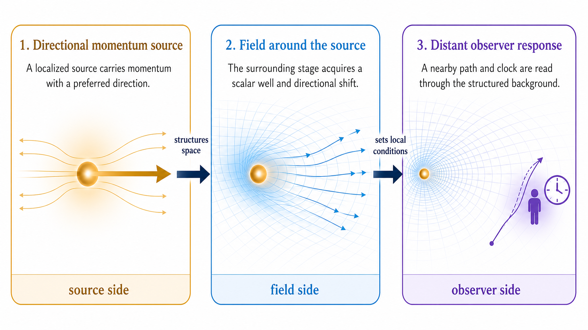
The deformation acts as a kinematic modifier: a physical structural effect that changes how a particle’s momentum configuration produces motion. Gravity is the first such modifier explored in M1; later chapters will also explore spatial expansion and the Pauli exclusion principle.
Now, light has no massive internal cycle to dilate, yet it still crosses the deformed space. Its local speed remains \(c\) while its direction can change along the path. Explaining gravity therefore requires both the internal response of massive particles and propagation through the surrounding geometry.
The interaction must also return to the source. The particles that respond to gravity also contribute to gravity themselves. As spatial dilation reduces the momentum required by their fermic cycles, momentum relocates into their bosonic structure and participates in translation. Their gravitational contribution must therefore be evaluated from this changed momentum configuration. Evolving spatial deformation also participates in the momentum balance. Its contribution can be negligible in most approximations. Source, space and responding particles must therefore participate in one reciprocal account. A prescribed background can be useful for calculating a trajectory, but the complete conservation test requires the momentum changes on both sides.
This chapter develops a model of that interaction and follows it through to clock comparisons, massive motion and light bending. The directional conservation algebra specifies the required balance; completing that account for a full curved gravitational system remains open. The source and response laws supply concrete consequences to compare with Newtonian gravity and general relativity.
3.2 Core Terms and Variables
The notation distinguishes sources, spatial deformation, the map between local and reference descriptions, and the particles realized in that setting. Each domain has its own table. Within a table, the inputs come before the quantities built from them, with related components kept together. The label \(a\) identifies one particle, also called a carrier.
3.2.1 Gravitational sources
| Symbol | Name | Definition or role |
|---|---|---|
| Individual particles | ||
| \(M_a\) | Realized carrier core momentum | Positive local core of particle \(a\), including its internal and translational contributions. |
| \(p_a^i\) | Realized translation | Local spatial momentum, with \(p_{i,a}=\delta_{ij}p_a^j\). |
| \(p_{k,a}\) | Signed directional projection | \(p_{k,a}=\mathbf p_a\mathbin{\cdot}\hat{k}\) for an oriented unit direction \(\hat{k}\). |
| \(p_{k,a}^{\pm}\) | Opposed carrier readings | \(p_{k,a}^{\pm}=M_a\pm p_{k,a}/2\). |
| Source construction | ||
| \(j_a{}^{\mu\nu}\) | Single-carrier source kernel | \(j_a{}^{\mu\nu}=p_a^\mu p_a^\nu/M_a\), formed before aggregation. |
| \(\langle\cdot\rangle\) | Local source moment | Sum with nonnegative weights per physical volume in the declared source frame. |
| \(\mathcal J_k^{\pm}\) | Opposed source channels | \(\mathcal J_k^{\pm}=\langle\sum_a p_{k,a}^{\pm}\rangle\). |
| \(J^{\mu\nu}\) | Local momentum source tensor | Actual momentum content in a region of space, \(J^{\mu\nu}=\langle\sum_a j_a{}^{\mu\nu}\rangle\). |
| Content, direction and transport | ||
| \(\mathcal M\) | Additive source content | \(\mathcal M=\langle\sum_a M_a\rangle=J^{00}\). |
| \(\mathcal P^i\) | Directional source imbalance | \(\mathcal P^i=\langle\sum_a p_a^i\rangle=J^{i0}\). |
| \(\mathcal C^{ij}\) | Momentum transport | \(\mathcal C^{ij}=\langle\sum_a p_a^ip_a^j/M_a\rangle=J^{ij}\). |
Here \(p_a^\mu=(M_a,p_a^i)\) collects the local momentum components, and \(p_{\mu,a}=(-M_a,p_{i,a})\) lowers the index with the local signature. Lowercase \(j\) records one carrier; uppercase \(J\) records the aggregate. The calligraphic symbols distinguish population quantities from individual momenta. The blocks \(\mathcal M\), \(\mathcal P^i\) and \(\mathcal C^{ij}\) belong to one source tensor. Source and deformation use all-upper components; the coframe remains a mixed-index map.
The source moment is taken at one event, in one declared frame. It is not a direct sum of components at separated locations. The particle construction in §3.3 supplies the kinetic case. Internal transport, binding and supporting stresses need their own consistent contributions to the same source; they are not fixed by the free-particle sum alone.
3.2.2 Spatial deformation
| Symbol | Name | Definition or role |
|---|---|---|
| \(\theta^{\mu\nu}\) | Deformation tensor | Collects the common, directional and spatial stretch/shear components. |
| \(\theta^{00}\) | Common deformation component | Core-content response; sourced by \(\mathcal M\) in the weak-field equations. |
| \(\theta^{0i}\) | Directional deformation components | Temporal–spatial entries, with \(\theta^{i0}=\theta^{0i}\). |
| \(\theta^{ij}\) | Spatial stretch/shear block | Spatial components of the same deformation array. |
The array \(\theta\) describes deformation relative to a specified reference. Its primary all-upper form is symmetric; reference-metric lowering is a separate operation.
3.2.3 Local and reference geometry
| Symbol | Name | Definition or role |
|---|---|---|
| Conversion map | ||
| \(\phi^\mu{}_\nu\) | Operational map | Converts coordinate increments \(dx^\nu\) into local increments \(d\ell^\mu\). |
| \((\phi^{-1})^\mu{}_\nu\) | Inverse operational map | Converts local increments back into coordinate increments. |
| Components of the map | ||
| \(\phi^0{}_0\) | Temporal map component | Temporal conversion; weakly \(\phi^0{}_0\simeq1-\theta^{00}-\delta_{kl}\theta^{kl}\). Distinct from a physical clock’s cycle rate. |
| \(\phi^i{}_0\) | Spatial–temporal map components | Local spatial increments contributed by a coordinate-time increment. |
| \(\phi^i{}_j\) | Spatial map components | Convert coordinate spatial increments into local spatial increments. |
| Local increments and interval | ||
| \(d\ell^\mu\) | Local temporal and spatial increments | \(d\ell^\mu=\phi^\mu{}_\nu dx^\nu\); the temporal increment in time units is \(d\ell^0/c\). |
| \(g_{\mu\nu}\) | Metric shadow | Interval representation derived from \(\phi\); \(g^{\mu\nu}\) is its inverse. |
The map connects reference displacements to local geometry:
\[ d\ell^\mu=\phi^\mu{}_\nu dx^\nu, \qquad g_{\mu\nu}=\eta_{\alpha\beta}\phi^\alpha{}_\mu\phi^\beta{}_\nu. \tag{3.1}\]
The upper slot of \(\phi\) is local output and the lower slot is coordinate input; the inverse reverses that direction. Its components belong to one map, and \(g\) is derived from it, not independently chosen. The Stage-adapted form used below has \(\phi^0{}_i=0\). A material clock or ruler still needs a model of the motion or equilibrium that produces its readings.
3.2.4 Particle realization and internal cycles
| Symbol | Name | Definition or role |
|---|---|---|
| Particle identity and location | ||
| \(p_f\) | Intrinsic fermic momentum | Fixed identity scale; written \(p_{f,a}\) when identifying a particular particle. |
| \(x_a^\mu\) | Carrier event / trajectory | Position in the declared coordinates, where the deformation is evaluated; \(x^0=ct\). |
| \(u_a^\mu\) | Proper-time four-velocity | \(u_a^\mu=dx_a^\mu/d\tau_a\), with \(g_{\mu\nu}u_a^\mu u_a^\nu=-c^2\). |
| Realized momentum configuration | ||
| \(p_a^i\) | Realized translation | Local spatial momentum, with \(p_{i,a}=\delta_{ij}p_a^j\). |
| \(M_a\) | Realized carrier core momentum | Positive local core; the free-carrier approximation uses \(M_a=\sqrt{p_{f,a}^2+p_a^ip_{i,a}}\). |
| \(p_a^\mu,\ p_{\mu,a}\) | Carrier four-momentum | One momentum family in the declared frame; local \(p_a^0=M_a\). |
\(p_r^\mu\) | Reference-expressed four-momentum | \(p_r^\mu=\phi^0{}_0(p^\mu)_{\mathrm{local}}\), in the map’s local output axes with the common distant normalization. |
\(M_r=-p_0\) | Reference core | \(M_r=p_r^0=\phi^0{}_0M\); \(p_0\) is the temporal coordinate covector component. |
\(p_r\) | Reference-expressed translation | \(p_r=\sqrt{\delta_{ij}p_r^ip_r^j}\), the magnitude of the reference-expressed spatial momentum. |
\(p_{k,r}\) | Signed reference projection | \(p_{k,r}=\delta_{ij}k^ip_r^j\) for a unit direction in the same local output axes. |
\(p_{k,r}^{\pm}\) | Opposed reference-shell momenta | \(p_{k,r}^{\pm}=M_r\pm p_{k,r}/2\). |
\(p_{f,r}\) | Reference-expressed fermic momentum | \(p_{f,r}=\sqrt{M_r^2-p_r^2}=\phi^0{}_0p_f\); the local free-carrier shell retains \(p_f\) as its coefficient. |
Realization describes the particle’s actual momentum configuration and propagation in the local deformation. The free-carrier shell used below keeps the free-space reference \(p_f\) fixed and combines it with translation. Resolving a particle’s internal momentum and stresses requires its structural model. For nonzero lightlike carriers, \(p_f=0\) and \(M=|\mathbf p|>0\).
3.2.5 Indices, signs and units
Greek indices run over \(0,1,2,3\); Latin spatial indices run over \(1,2,3\). A repeated tensor index is summed once up and once down. The labels \(f\), \(r\), \(a\) and \(k\) instead mark the fermic slot, its reference expression, a carrier and a reading direction. Carriers are summed explicitly with \(\sum_a\); the label \(k\) in \(p_{k,a}^{\pm}\) is not summed.
Frames are stated where quantities are used. Local source components use \(\eta_{\mu\nu}=\operatorname{diag}(-1,1,1,1)\) and spatial components use \(\delta_{ij}\); coordinate components use \(g_{\mu\nu}\). This signature reverses the overall interval convention used in Foundations’ inertial correspondence without changing its positive momentum readings. Ordinary indices are retained in both frames, and \(\phi\) connects them. In \(\phi^i{}_j\), the upper and lower slots therefore belong to different bases despite both carrying spatial indices.
The individual quantities \(p_f\), \(p_{f,r}\), \(M\), \(M_r\), \(p_\mu\), \(p_r^\mu\) and \(j_a{}^{\mu\nu}\) have momentum units; \(u^\mu\) has velocity units. Source densities such as \(J\), \(\mathcal M\), \(\mathcal P\) and \(\mathcal C\) have momentum-per-volume units. The deformation coefficients \(\theta\), the map coefficients \(\phi\), and the metric coefficients \(g\) are dimensionless in the chosen length coordinates. The conventional gravity dictionary is reserved for §3.10.
3.3 Gravitational Sources
In M1, momentum deforms space by creating tension in the geometry of space. To describe this tension or the resulting deformation, we must first establish a description of the amount and state of momentum in space. The deformation caused by momentum is naturally anisotropic, and the description must respect this. A natural first step is therefore to describe the momentum content of a volume through six directional channels, in a similar fashion to the momentum components of a particle’s momentum shell. We denote these channels by \(\mathcal J_k^\pm\), where \(k\) labels an arbitrary reading direction. These provide a primary measure of how much momentum occupies a region of space and how it is directed.
We begin in the weak-field approximation, treating the source particles as having their flat-space momentum configurations. Their gravitationally altered configurations, needed for stronger-field sources, come later, once the particle response to deformed space has been introduced in §3.5.
3.3.1 Adding the directional shells
Choose three perpendicular axes at the source point. Their opposed directions give six readings of the same local momentum content. Along any oriented direction \(\hat{k}\), each particle supplies the familiar readings \(p_{k,a}^\pm=M_a\pm p_{k,a}/2\), with \(M_a=\sqrt{p_{f,a}^2+p_a^ip_{i,a}}\). Adding them gives the primary source channels
\[ \mathcal J_k^\pm =\left\langle\sum_a p_{k,a}^\pm\right\rangle. \tag{3.2}\]
The brackets turn the sum into a local density: each particle population is weighted by its number per unit volume, in the same frame. Both channels receive positive contributions, including from light. Reversing a particle’s motion exchanges its opposed readings; it does not subtract that particle from the source.
Figure 3.2 connects the shell readings to their source densities. The same particles contribute to both channels; the side panels show their accumulation for identical particles with the same orientation.
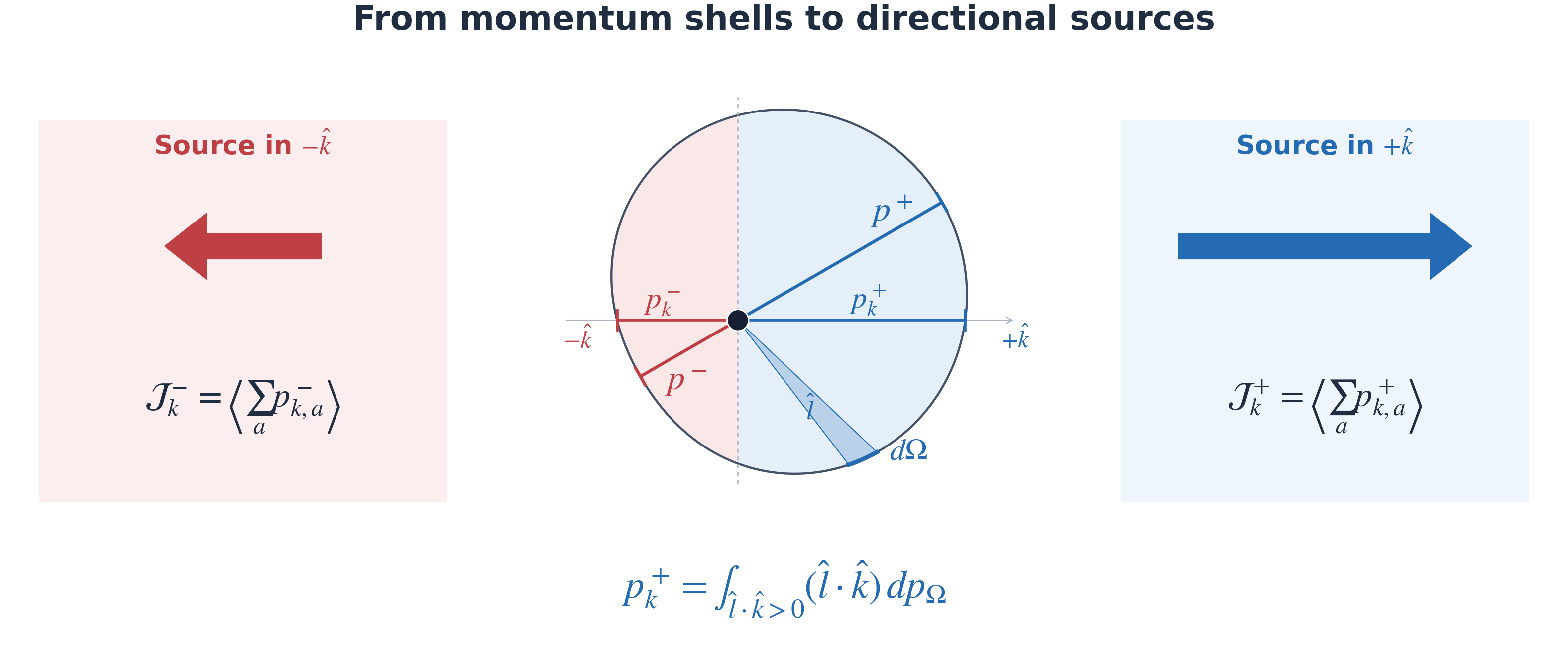
To separate how much momentum is present from which way it is directed, take the mean and difference of the channels:
\[ \begin{aligned} \mathcal M &=\frac{\mathcal J_k^++\mathcal J_k^-}{2} =\left\langle\sum_a M_a\right\rangle,\\ \mathcal P_k &=\mathcal J_k^+-\mathcal J_k^- =\left\langle\sum_a p_{k,a}\right\rangle. \end{aligned} \tag{3.3}\]
The mean \(\mathcal M\) is the same for every reading direction: it records the source’s additive core content. The difference \(\mathcal P_k\) records its directional imbalance and changes sign when the reading direction is reversed. Taking three spatial basis directions gives the components \(\mathcal P^i=\langle\sum_a p_a^i\rangle\).
A rotating body can have no net translational momentum and still have a directional source pattern. Figure 3.3 makes that pattern visible. Take the reading direction \(\hat{k}\) to the right. Particles in the upper half move against it, while particles in the lower half move along it. Their positive-channel contributions \(\mathcal J_k^+\) are consequently smaller above and larger below.
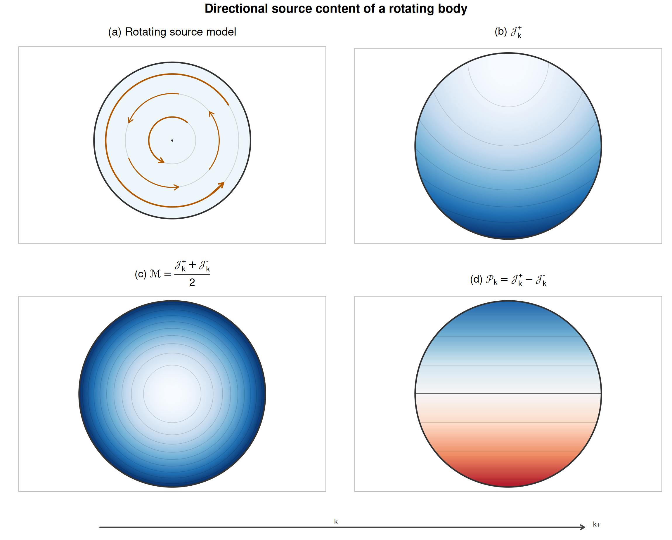
The channel mean in panel (c) removes that directional sign. Its circular contours reflect the larger core momentum of the faster-moving particles farther from the center. The difference in panel (d) instead changes sign across the body. Summing that difference over the whole body would erase precisely the spatial pattern that distinguishes rotation from rest.
3.3.2 Pressure and shear
Particles also carry momentum across space. This adds a secondary part of the source description: the pressure and shear associated with their motion. The transport tensor is
\[ \mathcal C^{ij} =\left\langle\sum_a\frac{p_a^ip_a^j}{M_a}\right\rangle. \tag{3.4}\]
The factor \(p_a^i/M_a\) is the particle’s velocity in direction \(i\) in units of \(c\). Multiplying it by \(p_a^j\) records the transport of momentum component \(j\) in that direction. For a population with no net local momentum, the diagonal entries give the kinetic normal stresses and the off-diagonal entries give the shear stresses. Equal diagonal entries describe isotropic pressure, expressed here in momentum-per-volume units.
This contribution comes from the same particle shells, but it retains information about how their individual momentum components occur together. The products must be formed particle by particle before averaging; they cannot generally be recovered from the summed channels alone.
For example, two equal streams, each with number density \(w\), core \(M\) and momentum \(\pm p\) along the first spatial axis give \(\mathcal J_k^+=\mathcal J_k^-=2wM\) for every \(k\), while \(\mathcal C^{11}=2wp^2/M\). Turn both streams onto the second axis: the primary source channels stay the same, but the transport moves to \(\mathcal C^{22}\). The primary channels retain their content and net imbalance; the transport tensor distinguishes the opposing flow patterns.
3.3.3 The momentum source tensor
The field equations need content, directional imbalance and transport together. The source tensor \(J^{\mu\nu}\) collects this actual momentum content in a region of space. For the particle population considered here, the local four-momentum \(p_a^\mu=(M_a,p_a^i)\) gives the single-particle contribution and its aggregate:
\[ j_a{}^{\mu\nu}=\frac{p_a^\mu p_a^\nu}{M_a}, \qquad J^{\mu\nu} =\left\langle\sum_a j_a{}^{\mu\nu}\right\rangle =\begin{bmatrix} \mathcal M&\mathcal P^j\\ \mathcal P^i&\mathcal C^{ij} \end{bmatrix}. \tag{3.5}\]
The division by \(M_a\) makes the temporal entries recover the particle’s core and spatial momentum, while the spatial block gives its momentum transport. Lowercase \(j_a\) records one particle’s contribution; uppercase \(J\) records the region’s momentum content. The all-upper array keeps \(J^{00}=\mathcal M\) positive and its directional entries symmetric. The kinetic array is positive semidefinite, although signed directional and shear entries need not be positive. Derivation 3.3A gives the resolved construction and its frame-dependent weights; here we use its flat-space particle limit.
In the weak field, the core content \(\mathcal M\) sources the common deformation \(\theta^{00}\). The transport trace also affects temporal readout, through the reconstruction of \(\phi\). The negative spacetime trace is a different combination. In the present source approximation,
\[ -\eta_{\mu\nu}J^{\mu\nu} =\mathcal M-\delta_{ij}\mathcal C^{ij} =\left\langle\sum_a\frac{p_{f,a}^2}{M_a}\right\rangle. \tag{3.6}\]
Subtracting the transport trace isolates the fermic contribution in this weighted form. Cold particles at rest make both combinations equal to \(\mathcal M\). Light has \(M=|\mathbf p|\) and hence \(\mathcal M=\delta_{ij}\mathcal C^{ij}\), while its temporal-readout combination is \(2\mathcal M\). A light bath can therefore have zero net direction and zero spacetime trace without ceasing to gravitate. Secondary transport is not necessarily small.
These formulas give the kinetic particle contribution. Binding, walls and supports require their own stresses; they cannot all be replaced by a sum of free streams. Deformation can carry momentum too. A complete gravitational account must include each contribution once, with its source representation supplied by consistent dynamics.
3.4 The Deformation of Space
Space has an underlying geometry. The exact description of this geometry is not yet established, but string theory does resonate strongly with the momentum structures we see. Exploration of this geometry will be carried out in part 0. For now, we will limit ourselves to describing the deformations.
With a description of the source in place, the next step is to describe how this geometry is deformed by momentum, and then connect that deformation to local displacement and cycling.
3.4.1 From source channels to deformation
The source tensor \(J^{\mu\nu}\) describes the actual momentum content in a region of space. A deformation can redistribute a particle’s fermic and bosic content. Its resulting momentum configuration enters \(J\) without changing the source definition.
The source content, directional imbalance and momentum transport enter different components of the surrounding deformation. In the weak stationary field law, \(\mathcal M\) contributes to the common deformation \(\theta^{00}\), while the local imbalance \(\mathcal P^i\) sources the temporal–spatial components \(\theta^{0i}\). The secondary transport tensor \(\mathcal C^{ij}\) supplies spatial stretch and shear, and its trace contributes to temporal readout through \(\phi\).
For a localized, conserved stationary leading source, with the deformation’s own stress negligible at this order and the fields vanishing at infinity, the aligned harmonic-coordinate response is
\[ \theta^{\mu\nu}(\mathbf r) =\frac{G_N}{c^3}\int \frac{J^{\mu\nu}(\mathbf r')} {|\mathbf r-\mathbf r'|}\,d^3\mathbf r'. \tag{3.7}\]
Every source component supplies the corresponding deformation component with the same coupling. Expanding the source into the blocks defined in §3.3 gives
\[ \begin{aligned} \theta^{00}(\mathbf r) &=\frac{G_N}{c^3}\int \frac{\mathcal M}{|\mathbf r-\mathbf r'|}\,d^3\mathbf r',\\ \theta^{0i}(\mathbf r) &=\frac{G_N}{c^3}\int \frac{\mathcal P^i}{|\mathbf r-\mathbf r'|}\,d^3\mathbf r',\\ \theta^{ij}(\mathbf r) &=\frac{G_N}{c^3}\int \frac{\mathcal C^{ij}}{|\mathbf r-\mathbf r'|}\,d^3\mathbf r'. \end{aligned} \tag{3.8}\]
Here \(G_N\) is the coupling of the adopted field law, and all source quantities are evaluated at \(\mathbf r'\). The inverse-distance kernel carries their spatial pattern into the surrounding deformation. Reversing the rotation reverses \(\mathcal P^i\) and its directional response, while leaving \(\mathcal M\) and the kinetic transport unchanged. A stationary rotating body also needs the stresses that sustain its motion; these must be included in its source.
3.4.2 From deformation to local increments
The registered deformation determines the metric shadow used to construct local increments:
\[ \begin{aligned} g_{00}&=-1+2(\theta^{00}+\delta_{kl}\theta^{kl}),\\ g_{0i}&=-4\delta_{ij}\theta^{0j},\\ g_{ij}&=(1+2\theta^{00}-2\delta_{kl}\theta^{kl})\delta_{ij} +4\delta_{ik}\delta_{jl}\theta^{kl}. \end{aligned} \tag{3.9}\]
These components reconstruct the operational map \(\phi\). We fix the local spatial axes by taking \([\phi^i{}_j]=[g_{ij}]_+^{1/2}\), the symmetric positive-definite square root. Its spatial Gram matrix then reproduces \(g_{ij}\), while the temporal and mixed blocks complete the same map. This frame choice leaves the sourced temporal–spatial components intact. We use the regular domain with a positive spatial metric and future temporal coefficient \(\phi^0{}_0>0\).
With weak deformation in this frame, the map reduces to
\[ \begin{aligned} \phi^0{}_0&\simeq1-\theta^{00}-\delta_{kl}\theta^{kl}, \qquad \phi^0{}_i=0,\\ \phi^i{}_0&\simeq-4\theta^{0i},\\ \phi^i{}_j&\simeq (1+\theta^{00}-\delta_{kl}\theta^{kl})\delta^i{}_j+2\delta_{jl}\theta^{il}. \end{aligned} \tag{3.10}\]
The temporal coefficient converts a coordinate-time increment into a local temporal increment. The mixed components contribute local spatial increments from that same coordinate-time increment; the spatial block converts coordinate displacements. In the registered convention \(\theta^{10}=\theta^{01}\), so the corresponding directional map is \(\phi^1{}_0\simeq-4\theta^{10}\).
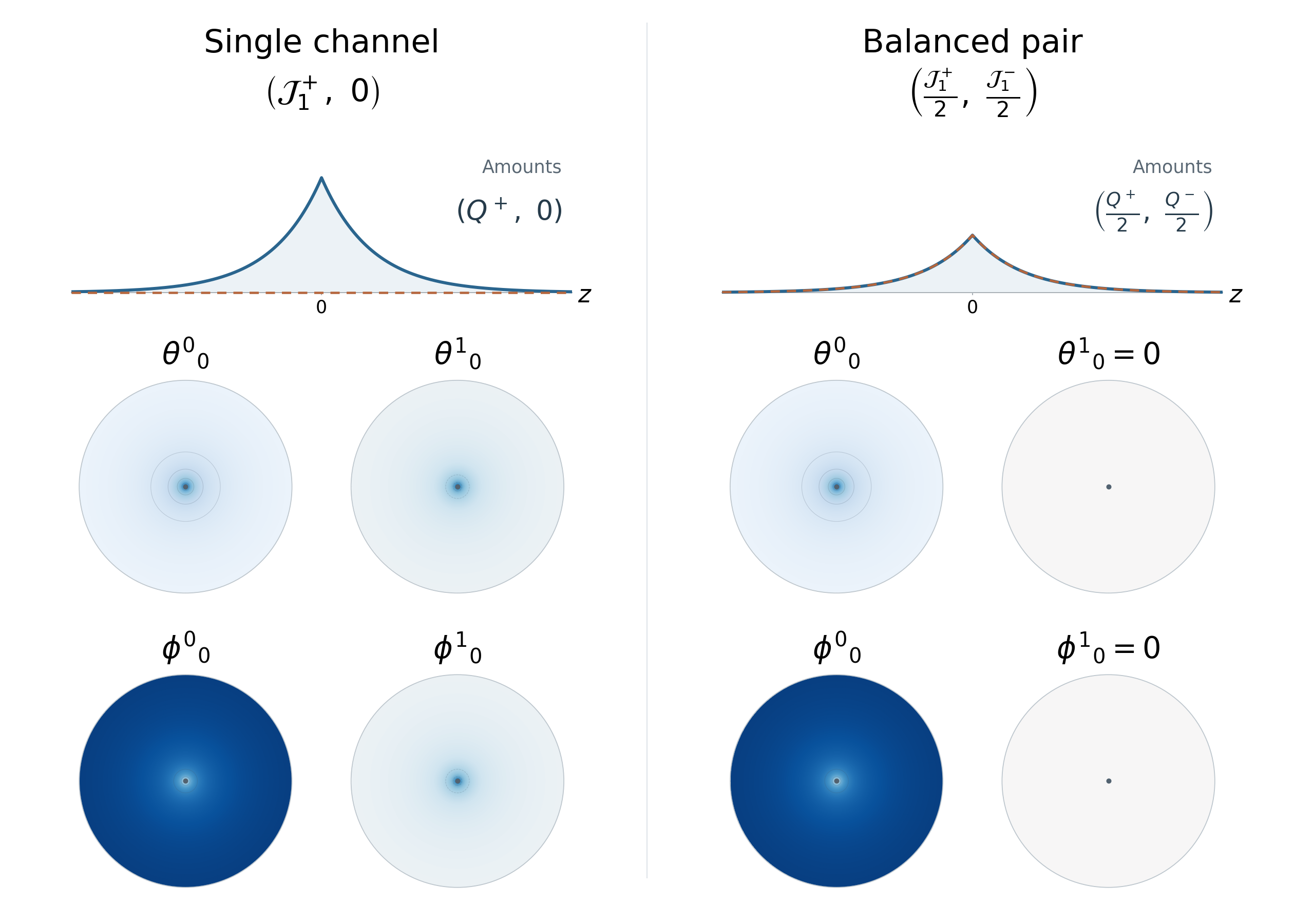
The linear response can be assembled one channel at a time. Take matched profiles in opposite directions, \(\mathcal J_1^+\) and \(\mathcal J_1^-\), with equal positive amounts \(Q^+\) and \(Q^-\):
\[ Q^\pm=\int\mathcal J_1^\pm(\mathbf x)\,d^3\mathbf x, \qquad Q^+=Q^->0. \tag{3.11}\]
Both profiles use the axial shape \(f(z)=e^{-|z|/r_0}/(2r_0)\), normalized to unit integral. Figure 3.4 compares the full positive-channel profile with half of each opposed profile. The respective amounts are \((Q^+,0)\) and \((\tfrac{Q^+}{2},\tfrac{Q^-}{2})\). Their sum is unchanged; their difference cancels. The figure isolates these channel contributions to the weak external map, keeping the transport contribution separate.
3.4.3 The sourced equations
For the external deformation, the model retains Einstein metric dynamics as an explicit physical input. This is a choice of field law, not a derivation of that law from ADMC. In native source notation,
\[ G^{\mu\nu}[g(\phi)] =\frac{8\pi G_N}{c^3}\bigl(J^{\mu\nu}\bigr)_{\mathrm{coord}}. \tag{3.12}\]
Here \(G^{\mu\nu}\) is the Einstein curvature operator of the metric shadow. Both indices of the displayed curvature operator are raised with the coordinate metric. The source is expressed in all-upper coordinate components: the conversion from the local source frame is \(J_{\mathrm{coord}}=\phi^{-1}J_{\mathrm{local}}\phi^{-\mathsf T}\). This changes the representation of the source, not its momentum content. The constant \(G_N\) belongs to this metric law. Each source contribution has momentum-per-volume units.
A solution also needs initial and boundary data. A changing configuration requires the initial deformation, its dynamical data and a compatible carrier population. A stationary exterior requires interior matching and whatever stresses maintain the source. The equations do not turn a prescribed body into a self-supporting one.
Derivation 3.4A constructs the finite map and obtains the free-carrier source from the same action used for motion in §3.5. A resolved material source also needs the internal and supporting stresses of its own particle model.
3.4.4 A weak spherical source
A simple exterior makes the source-to-deformation step concrete. Take a spherical body of radius \(R_s\), dominated by cold, slowly moving carriers with weak binding and small support corrections. Let \(M_{\mathrm{src}}\) be its integrated leading core content and define the length coefficient
\[ \ell_g=\frac{G_NM_{\mathrm{src}}}{c^3}. \tag{3.13}\]
Normalize the distant reference by \(\phi^0{}_0\to1\) and \(\phi^i{}_j\to\delta^i{}_j\). Outside the body, at the retained weak order,
\[ \begin{aligned} \phi^0{}_0(r)&\simeq1-\frac{\ell_g}{r},\\ \phi^i{}_j(r)&\simeq\left(1+\frac{\ell_g}{r}\right)\delta^i{}_j, \qquad \phi^0{}_i=\phi^i{}_0=0. \end{aligned} \tag{3.14}\]
The temporal coefficient is smaller near the source, while the spatial map stretches coordinate displacements into local lengths. In this nonrotating, orientation-aligned example \(\theta^{00}\simeq\ell_g/r\), with the other registered deformation components zero. The spatial map still changes because it depends on the full dictionary in Equation 3.9.
The approximation requires \(\ell_g/R_s\ll1\), small transport and binding/support corrections to the leading source, and observations in the exterior, with \(r\gg R_s\). Interior matching and the stresses that maintain the body are supplied, not solved. Derivation 3.4A gives the weak exterior construction. The weak exterior motion and light comparisons retain these assumptions; effects smaller than the omitted source or nonlinear corrections are not resolved by them. The later finite-geometry and material examples state their own source laws and regimes.
3.5 Particles in Deformed Space
A particle entering deformed space responds through both its motion and its internal structure. Expansion of the internal fermionic geometry lowers its realized fermic momentum. As the particle falls freely through a stationary gravitational well, momentum redistributes between the fermionic and bosonic structures while its reference core remains conserved.
3.5.1 The directional momentum shell
A particle’s four-momentum determines its entire directional momentum shell. The core fixes the shell’s mean, while the bosic momentum sets the difference between opposed directions.
Keep a static observer far from the well, where the map approaches the identity, and a static, zero-shift geometry with \(\phi^0{}_i=\phi^i{}_0=0\) and \(\phi^0{}_0>0\). Let \(p_f\) denote the particle’s fermic momentum in its free-space realization, taken as the undeformed reference for this comparison.
For a massive free carrier, write its future-directed four-velocity as \(u^\nu=dx^\nu/d\tau\), where \(\tau\) is geometric proper time along its path. Its normalization is \(g_{\mu\nu}u^\mu u^\nu=-c^2\). The map converts this coordinate four-velocity into local components. Expressing the corresponding momentum in the distant normalization gives
\[ p_r^\mu[\phi,u] =\frac{p_f\phi^0{}_0}{c}\phi^\mu{}_\nu u^\nu. \tag{3.15}\]
The upper index of \(p_r^\mu\) labels the fixed local axes of the map; the common factor \(\phi^0{}_0\) puts all components in the distant normalization. Extract the core and the signed bosic projection along a unit spatial direction \(k\), with \(\delta_{ij}k^ik^j=1\) in those same axes:
\[ M_r=p_r^0, \qquad p_{k,r}=\delta_{ij}k^i p_r^j. \tag{3.16}\]
In particular, \(M_r=\phi^0{}_0M=-p_0\), where \(M\) is the local core and \(p_0\) is the coordinate covector component. The opposed shell momenta are
\[ \boxed{ p_{k,r}^{\pm} =p_r^0\pm\frac12\delta_{ij}k^i p_r^j. } \tag{3.17}\]
Substituting the four-momentum gives the shell directly from the deformation map and the particle’s four-velocity:
\[ \boxed{ p_{k,r}^{\pm}[\phi,u] =\frac{p_f\phi^0{}_0}{c} \left(\phi^0{}_\nu \pm\frac12\delta_{ij}k^i\phi^j{}_\nu\right)u^\nu. } \tag{3.18}\]
For the 2D drawing, take a plane containing the bosic momentum and measure \(\alpha\) from its direction. The full outline is the polar plot
\[ R(\alpha)=M_r+\frac{p_r}{2}\cos\alpha, \qquad p_r=\sqrt{\delta_{ij}p_r^i p_r^j}. \tag{3.19}\]
Here \(R\) is only the plotted momentum radius, not a new physical field. The forward and backward values are \(M_r\pm p_r/2\), while every exactly perpendicular value is \(M_r\). At rest, \(p_r=0\) and the outline is a circle.
The core circle has radius \(M_r\). The fermic circle has radius
\[ p_{f,r}=\sqrt{M_r^2-p_r^2}=\phi^0{}_0p_f. \tag{3.20}\]
These relations reconstruct the directional momentum shell and its two reference circles. They do not determine a unique microscopic momentum density or a physical particle boundary.
3.5.2 At rest in the well
Compare two realizations of the same particle: one at rest far from a static source, the other settled at rest in the well. With no translation, \(p_r=0\). The realized fermic and core momenta therefore coincide:
\[ p_{f,r}=M_r=\phi^0{}_0p_f=\phi^0{}_0M. \tag{3.21}\]
Far away, where the map approaches the identity, the particle is realized with \(M=p_f\). In the well, \(\phi^0{}_0<1\) gives less realized fermic momentum and a smaller core in the same comparison.
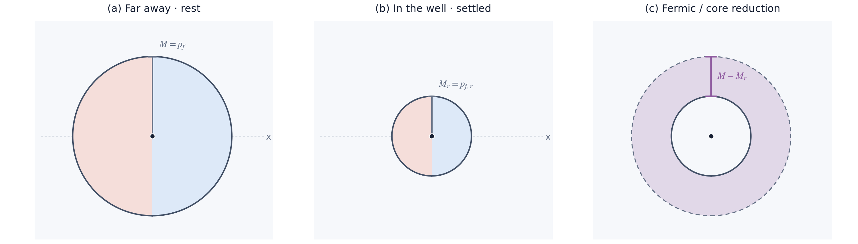
The purple area shows the fermic reduction between these resting states.
3.5.3 Motion and directional momentum
A moving carrier also carries directed bosic momentum. The fermic circle, core circle and full directional outline can therefore be distinguished.
Compare two such realizations at the same reference velocity. For translation along \(+x\) with a diagonal spatial map,
\[ \frac{v}{c} =\frac{\phi^0{}_0}{\phi^1{}_1}\frac{p_r}{M_r}. \tag{3.22}\]
A smaller temporal coefficient and a larger spatial coefficient reduce the velocity produced by a given bosic-to-core ratio. To match the distant particle’s reference velocity, the particle in the well therefore needs a larger ratio. In the example below, it has more reference-expressed bosic momentum even though its reference core is smaller.
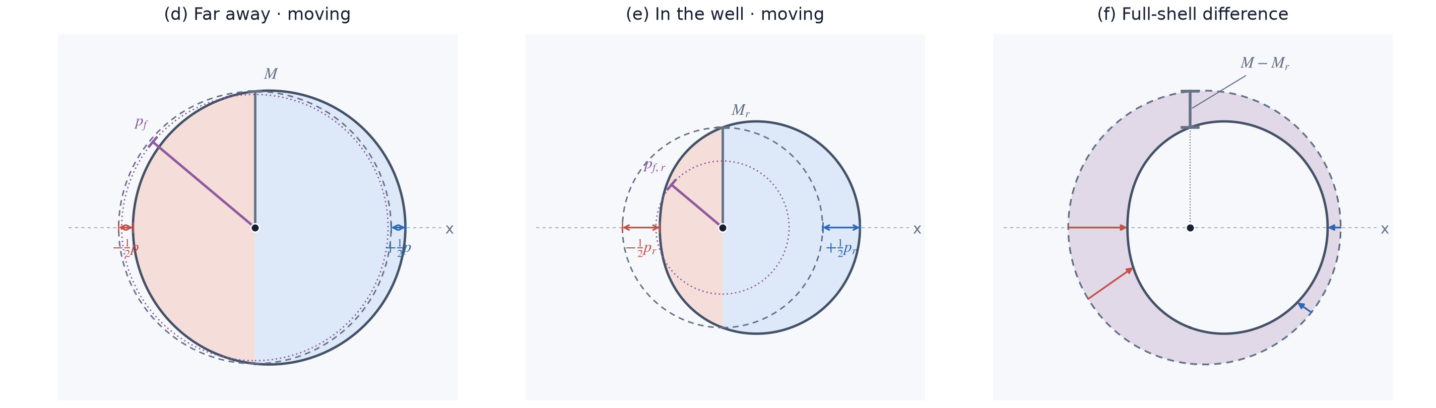
The unequal gaps around panel (f) show why the moving comparison is more than a uniform reduction. Perpendicular to the motion, the gap is \(M-M_r\). Along other directions it also contains the change in bosic imbalance.
3.5.4 Free fall, then settling
A freely falling particle changes its momentum configuration under a different condition: its reference core is conserved. Release it from rest in the distant limit. Stationarity fixes \(M_r=p_f\) along the free trajectory, and the reference budget gives
\[ M_r=p_f, \qquad p_r=p_f\sqrt{1-[\phi^0{}_0]^2}. \tag{3.23}\]
As the particle enters a deeper part of the well, \(p_{f,r}\) decreases and \(p_r\) grows. The dashed core circle stays fixed while the directional outline changes. Its local core rises according to \(M=M_r/\phi^0{}_0\); it is the common-reference core, not the local one, that is conserved.
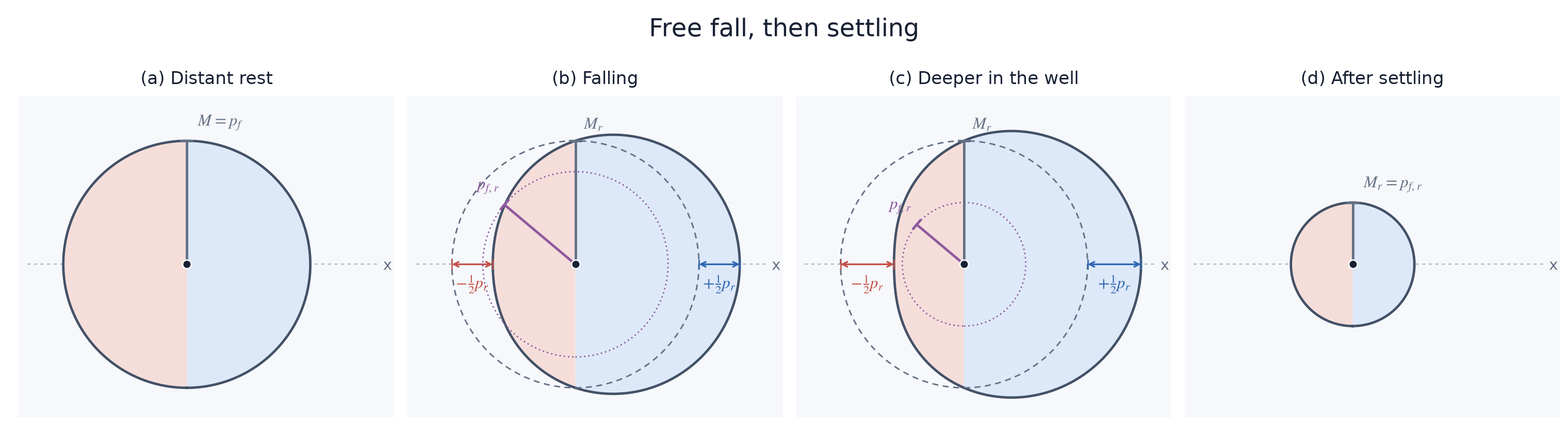
Settling removes the acquired translation. At the same depth, the final state has \(p_r=0\) and \(M_r=p_{f,r}\). The difference \(p_f-p_{f,r}\) is transferred to the surroundings. A particle settled in the well is therefore not the outcome of free fall alone: an interaction must remove core momentum as it stops the particle.
This example follows translational bosic momentum. In a structured particle, internal compensation need not all become centre-of-mass motion; its internal transport and supporting stresses require a structural model. Derivation 3.5A derives the free-carrier motion law, reference budget and stationary conservation.
3.5.5 Internal cycles and clocks
A clock counts a repeatable internal cycle. Let \(\varphi\) mark progress around a fermic cycle, with \(2\pi\) corresponding to one recurrence. For the ideal clock used here, held at rest with its cycle undisturbed by the support, take the cycling rate in the common reference to be
\[ \left(\frac{d\varphi}{dt}\right)_{\mathrm{held}} =\frac{cp_{f,r}}{\hbar} =\frac{cp_f}{\hbar}\phi^0{}_0. \tag{3.24}\]
The realized fermic scale sets this resting rate. Motion adds the slowing factor established in Foundations: the ratio of fermic momentum to core momentum. In the common reference that ratio is \(p_{f,r}/M_r=p_f/M\), so the moving cycle rate is
\[ \frac{d\varphi}{dt} =\frac{cp_{f,r}}{\hbar}\frac{p_{f,r}}{M_r} =\frac{c}{\hbar}\frac{p_{f,r}^{\,2}}{M_r}. \tag{3.25}\]
The dotted fermic circle and dashed core circle now connect the momentum configuration to physical cycling. A lower fermic scale slows the resting cycle; a larger core relative to that scale slows it further through motion.
At a fixed depth, settling removes the translational slowing, while the gravitational difference from the distant resting clock remains. Applying this ideal-cycle comparison to a particular material clock requires the internal dynamics and support conditions that keep its cycle stable. Section 3.10 turns the rate into a counted-pulse experiment.
3.5.6 Light in deformed space
Light has no fermic internal cycle: \(p_f=0\). Its momentum shell has \(M_r=p_r\) and \(p_{f,r}=0\). The local shell is \(M=|\mathbf p|\), and the null momentum relation gives
\[ -p_0=\phi^0{}_0\sqrt{g^{ij}p_ip_j}. \tag{3.26}\]
In stationary space this reference momentum is conserved along the ray. The local core can still vary, and the direction changes as the ray crosses the spatially varying map. Locally the speed is \(c\); a reference-coordinate path can nevertheless bend. Clock slowing and light bending therefore probe different aspects of the same deformation.
3.6 Reciprocal Sources
Every source particle exists in deformed space. A single particle will deform space locally, and its momentum configuration is, hence, never truly that of “free space”. To determine its actual momentum shell, we must account for both its motion and the deformation at its location. That shell supplies its contribution to \(J\).
3.6.1 The source contribution of realized particles
Continue with the free carriers in §3.5’s static, zero-shift geometry. Their momenta were expressed in a common distant reference, whereas the source formula of §3.3 uses local components. The conversion is \(p_r^\mu=\phi^0{}_0p_{\mathrm{local}}^\mu\), with \(M_r=\phi^0{}_0M\). Expressing the particle source in these reference quantities gives
\[ j_a^{\mu\nu} =\frac{p_{r,a}^{\mu}p_{r,a}^{\nu}} {\phi^0{}_0M_{r,a}}, \qquad J^{\mu\nu} =\left\langle\sum_a \frac{p_{r,a}^{\mu}p_{r,a}^{\nu}} {\phi^0{}_0M_{r,a}}\right\rangle. \tag{3.27}\]
The brackets average the particle contributions over physical volume in the local frame. The factors of \(\phi^0{}_0\) convert the reference momenta back to the local components used by the source.
For a massive particle, \(p_{r,a}^\mu\) follows from the deformation map and its motion, as derived in §3.5. The source formula is unchanged; the particles now contribute their momenta in deformed space.
3.6.2 The exact temporal feedback
Core momentum and momentum transport both source the temporal factor \(\phi^0{}_0\). In the static geometry, the field law of §3.4 gives
\[ D_iD^i\phi^0{}_0 =\frac{4\pi G_N}{c^3}\phi^0{}_0 \left(\mathcal M+\delta_{ij}\mathcal C^{ij}\right). \tag{3.28}\]
Here \(D_i\) is the spatial covariant derivative for \(g_{ij}\), so the operator follows the deformed spatial geometry. The equation applies at finite field strength.
For the free-particle population, its source term can be written directly in the reference momenta:
\[ \phi^0{}_0\left(\mathcal M+\delta_{ij}\mathcal C^{ij}\right) =\left\langle\sum_a\left( M_{r,a}+\frac{\delta_{ij}p_{r,a}^ip_{r,a}^j}{M_{r,a}} \right)\right\rangle. \tag{3.29}\]
Both the core and the directed transport of §3.5’s shell therefore enter the temporal field equation. For identical resting particles with local number density \(n\), the kinetic terms reduce to \(\mathcal M=np_f\) and \(\mathcal C^{ij}=0\), giving
\[ D_iD^i\phi^0{}_0 =\frac{4\pi G_N}{c^3}np_f\phi^0{}_0 =\frac{4\pi G_N}{c^3}np_{f,r}. \tag{3.30}\]
The local fermic density is \(np_f\); the field equation weights it by \(\phi^0{}_0\), giving \(np_{f,r}\). Derivation 3.6A obtains this weighting from the full field equation.
3.6.3 A supported reciprocal solution
In a static sphere, a pressure gradient balances gravity, and the pressure also contributes to the source. A constant-density continuum gives one exact example. Let its total local core density be \(\mathcal M_0\), with isotropic spatial stress. Define its radius \(R_s\) by the surface area \(4\pi R_s^2\). The length \(r_s=8\pi G_N\mathcal M_0R_s^3/(3c^3)\) sets the strength of its exterior field. With vanishing stress at the surface, the full static equations give the interior temporal map
\[ \phi^0{}_0(r) =\frac12\left[3\sqrt{1-\frac{r_s}{R_s}} -\sqrt{1-\frac{r_s r^2}{R_s^3}}\right], \qquad 0\leq r\leq R_s. \tag{3.31}\]
Derivation 3.6A solves the spatial map and supporting pressure along with this temporal map. A positive central clock factor and finite central support require \(r_s/R_s<8/9\). The spatial deformation and the pressure that balances the body are parts of the same solution.
3.6.4 A simplified scalar feedback model
To isolate the source reduction, prescribe a uniform resting population inside a sphere of radius \(R_s\), with \(n\) counted per Euclidean volume. As an additional scalar field-law postulate, extend the flat Poisson operator to finite deformation and source it with the reduced fermic content. Using \(\phi^0{}_0=\sqrt{1-2\theta^{00}}\) in this model gives
\[ \frac1{r^2}\frac{d}{dr}\left(r^2\frac{d\theta^{00}}{dr}\right) =-\frac{4\pi G_Nnp_f}{c^3}\sqrt{1-2\theta^{00}}. \tag{3.32}\]
A regular centre and continuous matching to a decaying exterior determine the profile. For the dimensionless source strength \(4\pi G_Nnp_fR_s^2/c^3=1\), the central and surface temporal factors are approximately \(0.58138\) and \(0.74031\), and the integrated source is \(0.67791\) of the unreduced value. The unexpanded square root makes the feedback explicit: increasing the well depth reduces the source that deepens it.
A related analytical example appears in Einstein’s self-coupled scalar gravity, discussed by Giulini: a uniform sphere has a reduced active mass and a hyperbolic-function interior solution. Derivation 3.6A compares that model with the scalar postulate used here.
Particle motion changes the source, the source changes the geometry, and the geometry changes the subsequent motion and source again. Following this feedback in time requires the full evolution equations for the source and deformation.
3.7 Field Equations
A changing source changes the space through which it moves. The stationary source integral of §3.4 describes a weak field with no time dependence. To follow a travelling disturbance, or the effect of a finite deformation on its own evolution, we use the differential field law introduced in §3.4.
3.7.1 The finite field law
The deformation \(\theta\) determines \(g\) and the local map \(\phi\) through §3.4’s relations. With the Einstein curvature operator chosen there, the field equation is
\[ G^{\mu\nu}\!\left[g(\theta)\right] =\frac{8\pi G_N}{c^3}J_{\mathrm{coord}}^{\mu\nu}, \qquad J_{\mathrm{coord}}^{\mu\nu} =(\phi^{-1})^\mu{}_\alpha (\phi^{-1})^\nu{}_\beta J^{\alpha\beta}. \tag{3.33}\]
The inverse map converts the local components of \(J\) into the coordinate components required by the field equation. On the left, \(G^{\mu\nu}\) combines spatial and temporal variations of the geometry. Since \(g\) is determined by \(\theta\), this is a field equation for the registered deformation.
Derivatives of \(g[\theta]\) first give the compatible connection, which relates local frames at neighboring points. Curvature then combines derivatives and products of that connection. The resulting operator contains second derivatives of \(\theta\), products of field gradients, and coefficients set by the finite geometry. Derivation 3.7A gives its explicit form and source normalization.
3.7.2 From the finite equation to propagation
For a weak deformation about the undeformed reference, choose coordinates satisfying \(\partial_\mu\theta^{\mu\nu}=0\) to leading order. The equation reduces to
\[ \Box\theta^{\mu\nu} =-\frac{4\pi G_N}{c^3}J^{\mu\nu}, \qquad \Box=-\partial_0^2+\delta^{ij}\partial_i\partial_j. \tag{3.34}\]
Since \(x^0=ct\), the temporal and spatial derivatives describe propagation at \(c\) in the undeformed reference. Removing the time dependence gives §3.4’s Poisson equation and its stationary source integral. Keeping it allows a source change to travel outward rather than alter the entire field instantaneously.
At finite deformation, the geometry determines the local propagation cone. The nonlinear terms also let one part of a gravitational disturbance influence another. The curvature operator already contains this gravitational self-coupling.
3.7.3 Initial data and constraints
To evolve a field, specify the geometry of a spatial slice, its rate of change, and the matter on it. The field equations link these initial data: their temporal projections constrain which combinations are possible. After the coordinates have been fixed, the remaining equations evolve the spatial geometry.
These constraints and the freedom to choose coordinates leave two local radiative polarizations among the ten symmetric components of \(\theta\). The fixed orientation of \(\phi\) specifies the local axes, while the connection relates frames at neighboring points.
A supported body needs its material equations as well as these gravitational equations. A population of free particles needs its transport law and initial distribution. Supplying \(J\) from the same matter dynamics that moves the source is what turns a field solution into a reciprocal one.
3.7.4 Momentum balance through the geometry
The field equation requires the local momentum balance
\[ \nabla_\mu J^{\mu\nu}=0. \tag{3.35}\]
This balance uses the connection of the evolving geometry. In coordinate components it reads
\[ \partial_\mu\!\left(\sqrt{-g}\,J^{\mu\nu}\right) =-\sqrt{-g}\,\Gamma^\nu{}_{\mu\alpha}J^{\mu\alpha}, \tag{3.36}\]
where \(g=\det(g_{\mu\nu})\). The right-hand side accounts for the changing comparison of momentum components between neighboring events. Coordinate components can therefore have changing volume integrals even while this local balance holds.
ADMC adds a global requirement: for an isolated system, the positive opposed directional totals must remain conserved in a declared common comparison. In a flat common frame, closed core and signed-momentum balances, together with \(\mathcal M\geq|\boldsymbol{\mathcal P}|\), give
\[ \int_V\mathcal J_k^\pm\,d^3x =\int_V\left(\mathcal M \pm\frac12\hat{k}\mathbin{\cdot}\boldsymbol{\mathcal P}\right)d^3x. \tag{3.37}\]
Derivation 3.7A obtains these conserved positive totals for closed boundaries. In curved space, a common directional balance also needs a way to compare separated local axes and to include the momentum carried by deformation, support and boundary transport. Constructing that complete account remains open.
3.8 Time-Dependent Gravity
Moving particles change the momentum source, and a changing deformation alters their subsequent motion. When both evolve, gravity is no longer a sequence of stationary wells. The particle distribution and the geometry must advance together.
3.8.1 Momentum in a changing geometry
The free-particle law from §3.5 also applies to a changing geometry. In coordinate components it gives
\[ \frac{dx^i}{dx^0}=\frac{p^i}{p^0}, \qquad \frac{dp_\mu}{dx^0} =-\frac{1}{2p^0}\partial_\mu g^{\alpha\beta}p_\alpha p_\beta. \tag{3.38}\]
The second equation now includes changes in the temporal momentum:
\[ \frac{d(-p_0)}{dx^0} =\frac{1}{2p^0}\partial_0g^{\alpha\beta}p_\alpha p_\beta. \tag{3.39}\]
In a stationary geometry, \(\partial_0g^{\alpha\beta}=0\) and \(-p_0\) is conserved. Time dependence allows \(-p_0\) to change according to the equation above. The conserved reference core in §3.5 followed from this time symmetry.
A collisionless population evolves by transporting particles through position and momentum space. Averaging their local contributions gives the changing \(J\). The same transport law implies \(\nabla_\mu J^{\mu\nu}=0\), so the motion that updates the source also preserves its local momentum balance.
3.8.2 A disturbance travels through space
In the weak regime, with no incoming radiation, the sourced solution is retarded:
\[ \theta^{\mu\nu}(t,\mathbf x) =\frac{G_N}{c^3}\int \frac{J^{\mu\nu}\!\left(t-|\mathbf x-\mathbf x'|/c,\mathbf x'\right)} {|\mathbf x-\mathbf x'|}\,d^3x'. \tag{3.40}\]
A change at the source reaches another point after a finite travel time. The stationary integral returns when the delay no longer changes the source values. Free gravitational radiation can be specified separately in the initial data.
In the weak vacuum, the equations admit two transverse wave polarizations. They change the tidal separation between neighboring free trajectories even when the common component \(\theta^{00}\) vanishes. Describing these waves requires the spatial components of the deformation, beyond a scalar well. At finite field strength, disturbances follow the local null cone of the evolving geometry.
Derivation 3.8A gives the transport and wave calculations. The full free-particle–field system has local evolution from regular, constraint-satisfying data under the conditions stated in Derivation 3.7A.
3.8.3 An exact coupled example
A uniform, isotropic population of light gives an exact coupled example. Choose a spatial map that stretches every direction by the same time-dependent factor:
\[ \phi^0{}_0=1, \qquad \phi^i{}_j=a(x^0)\delta^i{}_j, \qquad \phi^0{}_i=\phi^i{}_0=0, \tag{3.41}\]
Here \(a>0\) sets the physical distance between coordinate points. Translation symmetry keeps each particle’s coordinate momentum \(p_i\) fixed, while its local spatial momentum is \(p_i/a\). The number density per physical volume scales as \(a^{-3}\): the same population occupies a changing volume.
Normalize \(a(0)=1\) and let \(\mathcal M_0\) be the initial core density. Each nonzero light carrier has local core equal to its spatial momentum magnitude, so its core scales as \(a^{-1}\). Together with the changing number density, this gives
\[ \mathcal M=\mathcal M_0a^{-4}, \qquad \mathcal P^i=0, \qquad \mathcal C^{ij}=\frac{\mathcal M}{3}\delta^{ij}. \tag{3.42}\]
Solving the full field equations with this source gives the expanding solution
\[ a^2(x^0) =1+2\sqrt{\frac{8\pi G_N\mathcal M_0}{3c^3}}\,x^0. \tag{3.43}\]
The opposite sign before the time term gives the contracting solution. Both branches apply while \(a>0\). In each case, the particle trajectories, source and full field equations—constraints as well as evolution—are satisfied together.
The corresponding registered deformation is
\[ \theta^{00}=\frac{3(a^2-1)}8, \qquad \theta^{0i}=0, \qquad \theta^{ij}=\frac{1-a^2}{8}\delta^{ij}. \tag{3.44}\]
The common component and spatial trace cancel in the temporal map, leaving \(\phi^0{}_0=1\), while the spatial geometry evolves. Time derivatives now supply field terms that were absent from §3.6’s static equation. This example tests coupled gravitational evolution; the physical assumptions of the book’s separate expansion engine are introduced later.
3.8.4 A material recurrence can evolve too
An oscillating body provides a clock whose recurrence can be followed through changing geometry. Take a specified self-bound fluid model with a supported spherical equilibrium and a small radial oscillation. Finite perturbations make its surface move and its internal stresses evolve along with the gravitational field, so the period can shift from its linear value.
The numerical calculation follows two small but finite perturbations for six reference periods, with no signal probe present. At the larger amplitude, successive periods shorten slightly toward the linear value. The resolution study separates this change from numerical drift over the tested interval.
A time comparison must follow the moving surface as well. Its elapsed proper time is
\[ \Delta\tau_s =\int_{t_1}^{t_2} \sqrt{-g_{\mu\nu}(x_s(t)) \frac{dx_s^\mu}{c\,dt}\frac{dx_s^\nu}{c\,dt}}\,dt. \tag{3.45}\]
The integral accumulates gravitational and translational slowing along the actual surface motion. Both the geometry and the velocity must therefore be updated throughout the recurrence. This is the dynamical counterpart of §3.5’s clock comparison, now applied to an evolving material body.
§3.10 compares this material recurrence and a separate weak scalar-signal calculation with GR. Finite material–signal exchange has been evolved in a homogeneous model; coupling such an exchange to the oscillating body and a distant observer remains open.
3.9 Gravity in Six Directional Components
The directional shell does not begin with one time slot and three spatial slots. It begins with six positive directional components: one for each branch of three opposed axes. This is the more M1-native way to display the same gravitational content. The ordinary four-component form remains available, but the six-component form shows source correlations, metric comparison and transport relations directly.
3.9.1 Six readings, four degrees of freedom
Choose one local orthonormal frame. Let a slashed component index \(\not i\) label one of the six directional components,
\[ \not i\in\{1+,1-,2+,2-,3+,3-\}. \]
For a particle with core \(M\) and signed spatial components \(p_i\), the six directional components are
\[ p^{i\sigma}=M+\frac{\sigma}{2}p_i, \qquad i=1,2,3, \qquad \sigma=\pm1. \tag{3.46}\]
Equivalently, write these components as \(p^{\not i}\). The inverse relations are
\[ M=\frac16\sum_{\not i}p^{\not i}, \qquad p_i=p^{i+}-p^{i-}. \tag{3.47}\]
Thus the six readings contain the ordinary core and signed momentum in a supported four-dimensional pattern. Their opposed pair sums satisfy
\[ p^{1+}+p^{1-} =p^{2+}+p^{2-} =p^{3+}+p^{3-}=2M. \tag{3.48}\]
The pair-sum equalities define a four-dimensional supported subspace inside the six displayed components. Future carriers also obey the mass-shell condition \(M\geq|\mathbf p|\), so every directional component is positive. Using §3.5’s reference-expressed momenta gives the same six-component shell for particles in deformed space.
For comparison with the ordinary form, order the six components as \((1+,1-,2+,2-,3+,3-)\). Use \(L\) for both directions and let the indices state the direction of the map:
\[ p^{\not i}=L^{\not i}{}_{\mu}p^\mu, \qquad p^\mu=L^\mu{}_{\not i}p^{\not i}. \]
Here the ordered ordinary components are \(p^\mu=(M,p_1,p_2,p_3)^{\mathsf T}\) and the ordered six-component list is \((p^{1+},p^{1-},p^{2+},p^{2-},p^{3+},p^{3-})^{\mathsf T}\). In matrix form,
\[ [L^{\not i}{}_{\mu}]= \begin{pmatrix} 1&1/2&0&0\\1&-1/2&0&0\\ 1&0&1/2&0\\1&0&-1/2&0\\ 1&0&0&1/2\\1&0&0&-1/2 \end{pmatrix}, \qquad [L^\mu{}_{\not i}]= \begin{pmatrix} 1/6&1/6&1/6&1/6&1/6&1/6\\ 1&-1&0&0&0&0\\ 0&0&1&-1&0&0\\ 0&0&0&0&1&-1 \end{pmatrix}. \tag{3.49}\]
Lifting and returning leaves the ordinary four-component vector unchanged:
\[ L^\mu{}_{\not i}L^{\not i}{}_{\nu}=\delta^\mu{}_{\nu}. \]
The reverse contraction \(L^{\not i}{}_{\mu}L^\mu{}_{\not j}\) returns the six readings to the equal-pair-sum support. Derivation 3.9A gives the projector and supported metric forms.
3.9.2 The metric compares common content with opposed differences
The same sums and differences that recover core and bosic momentum also define the native reference metric. The core is the average of all six readings, while each bosic component is an opposed difference. The shell invariant is therefore
\[ \boxed{ \eta_{\not i\not j}p^{\not i}p^{\not j} =\sum_{k=1}^{3}\left(p^{k+}-p^{k-}\right)^2 -\left(\frac16\sum_{\not i}p^{\not i}\right)^2 =-p_f^2. } \tag{3.50}\]
This equation uses the local readings defined above. For the static reference readings \(p_r^{\not i}=Np^{\not i}\), the same contraction is instead \(-p_{f,r}^{\,2}=-(Np_f)^2\).
The metric combines directional imbalance and common content into one invariant. The minus sign distinguishes those roles; it does not introduce negative momentum content. Componentwise, using the same branch notation as \(p^{i\sigma}\), this is the supported reference metric:
\[ \boxed{ \eta_{i\sigma,j\tau} =\sigma\tau\,\delta_{ij} -\frac1{36}. } \tag{3.51}\]
The signs \(\sigma\) and \(\tau\) are \(+1\) on plus branches and \(-1\) on minus branches. The Kronecker delta compares the two spatial axes; there is no hidden sum over the displayed component labels.
The deformed Stage applies the same structure to geometric increments. The readout map gives
\[ d\ell^{\not i}=\phi^{\not i}{}_{\not j}dx^{\not j}. \tag{3.52}\]
The interval can then be written entirely in six-component language:
\[ \boxed{ g_{\not i\not j}dx^{\not i}dx^{\not j} =\sum_{k=1}^{3}\left(d\ell^{k+}-d\ell^{k-}\right)^2 -\left(\frac16\sum_{\not i}d\ell^{\not i}\right)^2. } \tag{3.53}\]
The rule is the same as for the momentum shell: compare the three opposed displacement differences with the common process increment. Deformation changes that comparison through \(\phi\). These increments are geometric quantities, and in the retained correspondence their common increment supplies the local clock component. Equivalently,
\[ g_{\not i\not j} =\eta_{\not k\not l}\, \phi^{\not k}{}_{\not i}\phi^{\not l}{}_{\not j}. \tag{3.54}\]
Source, shell and metric now share one organizing structure: common content plus opposed differences. The common mode carries the temporal role; the opposed differences carry the spatial roles. Metric coefficients can therefore have mixed signs even though the directed momentum readings themselves are positive.
3.9.3 Source correlations appear as component products
The source describes which directional components occur together. Form products for each carrier before averaging:
\[ J^{\not i\not j} =\left\langle\sum_a \frac{p_a^{\not i}p_a^{\not j}}{M_a}\right\rangle. \tag{3.55}\]
The six-by-six source records correlations between directional components. The aggregate first moments recover \(\mathcal M\) and \(\mathcal P^i\), but the transport block \(\mathcal C^{ij}\) depends on which directional readings occur together on the same carriers. Equal counterstreams along \(x\) and equal counterstreams along \(y\) can have the same core and zero net spatial momentum while transporting momentum in different directions.
For two equal carriers with momenta \(\pm p\hat x\) and local core \(M\), the opposed \(x\) components differ by
\[ J_x^{1+,1+}-J_x^{1+,1-}=\frac{p^2}{M}, \qquad J_x^{2+,2+}-J_x^{2+,2-}=0. \tag{3.56}\]
For equal streams along \(y\), the nonzero difference moves from the \(1\) pair to the \(2\) pair. The first moments are identical in the two cases; the component correlation shows which direction carries transport. Derivation 3.9A gives the calculation.
The ordinary source and the six-component source are connected by the same lift and recovery on both upper slots:
\[ J^{\not i\not j}=L^{\not i}{}_{\mu}L^{\not j}{}_{\nu}J^{\mu\nu}, \qquad J^{\mu\nu}=L^{\mu}{}_{\not i}L^{\nu}{}_{\not j}J^{\not i\not j}. \tag{3.57}\]
The deformation has the same supported dictionary:
\[ \theta^{\not i\not j}=L^{\not i}{}_{\mu}L^{\not j}{}_{\nu}\theta^{\mu\nu}, \qquad \theta^{\mu\nu}=L^{\mu}{}_{\not i}L^{\nu}{}_{\not j}\theta^{\not i\not j}. \tag{3.58}\]
The slashed components and the ordinary components are two views of the same supported object. A source written as \(J^{\not i\not j}\) displays how the opposed directional readings correlate; applying \(L^\mu{}_{\not i}\) to each slot returns the ordinary four-component source.
3.9.4 Curvature compares directional momentum between places
A source correlation asks which directional momenta occur together at one location. The geometric question is how the deformed Stage changes the comparison of those readings between neighboring locations. The connection supplies that comparison rule. Curvature measures its path dependence: transport the same momentum configuration along two infinitesimally different routes and compare the results.
In the fixed supported component basis,
\[ [\nabla_{\not k},\nabla_{\not l}]p^{\not i} =\mathcal R^{\not i}{}_{\not j\not k\not l}p^{\not j}. \tag{3.59}\]
The first two slots describe the momentum response; the last two describe the two transport directions. Curvature is an oriented change in transport, so reversing the path orientation reverses signs. The sign of a curvature component therefore records the orientation of comparison, not the presence of negative momentum content.
The field equation uses a particular two-index contraction of this transport curvature, the source-matched curvature response. In six-component form this response is the lifted two-index curvature combination
\[ G^{\not i\not j} \equiv L^{\not i}{}_{\mu}L^{\not j}{}_{\nu} \left(R^{\mu\nu} -\frac12 g^{\mu\nu}\,R\right), \tag{3.60}\]
For this finite coordinate-curvature equation, convert the local source first:
\[ J_{\mathrm{coord}}^{\mu\nu} =(\phi^{-1})^\mu{}_{\alpha}(\phi^{-1})^\nu{}_{\beta}J_{\mathrm{local}}^{\alpha\beta}, \qquad J_{\mathrm{coord}}^{\not i\not j} =L^{\not i}{}_{\mu}L^{\not j}{}_{\nu}J_{\mathrm{coord}}^{\mu\nu}. \]
The retained field law is
\[ L^{\not i}{}_{\mu}L^{\not j}{}_{\nu} \left(R^{\mu\nu} -\frac12 g^{\mu\nu}\,R\right) =\frac{8\pi G_N}{c^3}J_{\mathrm{coord}}^{\not i\not j}. \tag{3.61}\]
Both sides now use coordinate components and the same supported six-component representation. The equation constrains the source-matched contraction of curvature. The full transport curvature \(\mathcal R^{\not i}{}_{\not j\not k\not l}\) can still carry vacuum tidal structure and propagating disturbances where the local source term vanishes.
3.9.5 The weak solution component by component
In the aligned weak-harmonic limit,
\[ G^{(1)\not i\not j} =-2\Box\theta^{\not i\not j}, \tag{3.62}\]
so the field equation becomes
\[ \Box\theta^{\not i\not j} =-\frac{4\pi G_N}{c^3}J^{\not i\not j}. \tag{3.63}\]
For a localized conserved stationary source, this gives
\[ \theta^{\not i\not j}(\mathbf x) =\frac{G_N}{c^3}\int \frac{J^{\not i\not j}(\mathbf x')}{|\mathbf x-\mathbf x'|}\,d^3x'. \tag{3.64}\]
Each source correlation drives its corresponding deformation component in this weak limit. The finite operator then describes how all components jointly determine the comparison geometry through \(g\), the connection and its curvature. Applying \(L^\mu{}_{\not i}\) to both upper slots recovers the ordinary four-component equation and solution.
The six-component form brings the retained GR-equivalent dynamics into the language of M1’s directional momentum. Source correlations deform the Stage, the deformed Stage changes directional momentum comparison, and curvature records the path dependence of that comparison.
3.10 Correspondence with Newtonian Gravity and General Relativity
The field law used in this chapter reaches beyond the inverse-square force: it governs finite geometry, gravitational waves and changing sources. Its correspondence with GR therefore rests on the coupled equations, including the laws for matter and measurement. These determine both the exact agreement and where a different M1 law could change a prediction.
3.10.1 Exact agreement under the same physical laws
The source tensor uses momentum units. In the same frame, the conventional stress–energy tensor is
\[ T^{\mu\nu}=cJ^{\mu\nu}, \qquad m_0=\frac{p_f}{c}. \tag{3.65}\]
The second relation identifies the free carrier’s rest-mass parameter. In a zero-shift chart, GR’s lapse is \(N=\phi^0{}_0\) and its spatial metric is \(h_{ij}=g_{ij}\). The dictionary expresses the same source and geometry in conventional units and variables.
With this dictionary, the retained field equation is exactly
\[ G^{\mu\nu}[g]=\frac{8\pi G_N}{c^4}T^{\mu\nu}. \tag{3.66}\]
On the regular domain, the map between \(\theta\) and \(g\) is invertible and preserves all ten finite field equations. The free-carrier coupling gives the same timelike and null geodesics, and its distribution follows the same collisionless transport law. With the same matter laws, initial and boundary data, and measurement models, this sector gives exactly the same GR solutions and predictions.
The agreement includes the four initial constraints, two local gravitational-wave polarizations and null gravitational characteristics. Under the appropriate regularity conditions, local existence and uniqueness carry over for massive data, and separately for purely massless data supported away from zero momentum. Derivation 3.10A gives these conditions and the comparison premises.
3.10.2 One weak source, three familiar tests
For §3.4’s cold weak source, write \(m_{\mathrm{src}}=M_{\mathrm{src}}/c\) and \(\ell_g=G_Nm_{\mathrm{src}}/c^2\). A slow probe then has
\[ \mathbf a\simeq-\frac{G_Nm_{\mathrm{src}}}{r^2}\widehat{\mathbf r}. \tag{3.67}\]
This is the Newtonian inverse-square limit. The same source coefficient enters the clock and light comparisons, without separate adjustments of the gravitational coupling.
To turn §3.5’s ideal clock law into an experiment, hold identical clocks at \(a\) and \(b\) in a static zero-shift geometry, with supports that leave their cycles unchanged. Clock \(a\) sends one pulse every \(m\) cycles. Let \(\mathcal R_{a\to b}\) be the number of received pulses per cycle of clock \(b\). The stationary travel time shifts arrival times but not their separation, so
\[ m\mathcal R_{a\to b}=\frac{N_a}{N_b}, \qquad m\mathcal R_{a\to b}-1 \simeq-\ell_g\left(\frac1{r_a}-\frac1{r_b}\right). \tag{3.68}\]
With \(N_a<N_b\), the emitter runs more slowly than the receiver, which records a reduced pulse rate per cycle. The comparison is made through counted events.
For a distant light ray with impact parameter \(B\), the temporal and spatial maps together give
\[ \delta_{\mathrm{light}}\simeq\frac{4\ell_g}{B} =\frac{4G_Nm_{\mathrm{src}}}{c^2B}. \tag{3.69}\]
This is the leading GR deflection. Both temporal slowing and spatial deformation contribute to it. The same weak metric gives the propagation delay, while the finite metric and timelike geodesics give orbital precession. All these effects follow from one geometry and one probe coupling.
3.10.3 Finite geometry and horizons
At finite field strength, the supported constant-density solution of §3.6 is the interior Schwarzschild continuum expressed in momentum units. Its pressure, curved volume and temporal weighting enter together.
A complementary vacuum example passes through a horizon without a singular operational map. In ingoing Painlevé–Gullstrand coordinates, let \(r_s=2G_Nm_{\mathrm{src}}/c^2\) and \(r=|\mathbf x|>0\). The local intervals are
\[ d\ell^0=dx^0, \qquad d\boldsymbol\ell =d\mathbf x+\sqrt{\frac{r_s}{r}}\,\widehat{\mathbf r}\,dx^0. \tag{3.70}\]
This is the Schwarzschild vacuum in a freely falling local frame. Direct substitution satisfies the full field constraints and stationary evolution equations, including at \(r=r_s\). Radial null paths obey
\[ \frac{dr}{dx^0}=-\sqrt{\frac{r_s}{r}}\pm1, \tag{3.71}\]
while their speed in the local frame remains \(c\). A clock held at fixed coordinates moves relative to these freely falling frames; its exterior rate is \(\sqrt{1-r_s/r}\), although \(\phi^0{}_0=1\) in this shifted map. At the horizon that held worldline ceases to be timelike, while the map itself remains regular.
3.10.4 Complete sources and finite regions
A source must also represent the stresses of its material, including binding and support. For the free-particle source of §3.3,
\[ n_i\mathcal C^{ij}n_j =\left\langle\sum_a\frac{(n_ip_a^i)^2}{M_a}\right\rangle\geq0 \tag{3.72}\]
for every spatial direction \(n_i\). A free-particle population therefore has nonnegative normal stress in every direction. Matter with tension needs the stress contributions of its binding fields or internal dynamics as well.
The momentum balance of a finite region includes boundary transport, changes in physical volume and the comparison of local directions across the region. Integrating the local balance retains these flux and geometry terms. Explicit finite-window balances and error bounds quantify these effects. A spatial average alone therefore leaves out information needed for a closed source law.
3.10.5 A supported body with its own clock
A self-bound fluid model supplies a body with its own surface and support. Its pressure vanishes at a finite nonzero density, giving a free surface. Solving the material and gravitational equations together produces a regular spherical body that matches the exterior Schwarzschild geometry without a surface stress layer.
The body’s small radial displacements obey an oscillation equation derived from the same material law. In the worked models, an analytic positive bound on every admissible radial eigenvalue establishes linear radial stability. The fundamental mode provides a recurrence, and the changing surface area supplies its clock observable.
A specified weak scalar signal carries that material recurrence outward. The moving body generates sidebands above and below the carrier, each offset by the independently calculated material frequency. Changing the incident carrier frequency leaves those offsets unchanged, while a stationary-body control removes the sidebands. Thus the outgoing signal records the body’s cadence rather than a cadence prepared in the input.
For this effective material, support, source, recurrence and the weak outgoing scalar field follow from compatible laws. The calculation connects the body’s dynamics to a signal carrying its cadence. Electromagnetic detection and other material clocks require their own dynamical models.
3.10.6 What the dynamical calculations add
The nonlinear evolution in §3.8 advances the same body and its changing geometry for six periods at two specified finite perturbations, with the signal switched off. It measures successive periods and accumulated surface time from the evolved motion. The larger-perturbation extension remains outside the verified range: agreement of local and boundary balances is needed as well as a smooth surface trajectory.
The finite equations for the material and scalar together include opposite momentum exchange, propagated gravitational constraints and transmission across a moving material surface. At finite signal strength, scalar stress outside the body can change its surface mass. The exterior must then evolve along with the body and signal.
Finite material–scalar exchange with gravitational response has been demonstrated in a separate homogeneous calculation. The nonlinear bounded-body evolution, its weak outgoing-signal comparison and the homogeneous finite-exchange solution are distinct results. A full nonlinear body–signal–detector comparison still needs its own coupled solution.
3.10.7 Where M1 could differ
Agreement with GR is exact while the field, matter and measurement laws are shared. A genuine departure must therefore change one of those laws: how internal momentum is redistributed, how its stresses source space, how space evolves, or how a material clock and signal couple to that evolution.
Weak agreement does not uniquely choose the finite laws. Distinct nonlinear field equations can share a linear calibration, and distinct clock couplings can share a free-space frequency. A departure becomes a prediction only after its additional law is specified and its observable consequence derived. §3.6’s finite Poisson-feedback model makes one such additional field-law choice; its flat Poisson operator, Euclidean source-volume weights and scalar feedback define a different calculation from the full tensor solution.
M1 requires internal fermic-to-bosic compensation and complete directional conservation. Turning these requirements into a microscopic source and support law, with a consistent common-frame account in curved space, remains the native construction to be completed. The GR results provide its benchmark: a completion must reproduce the shared-law predictions or derive a testable departure from a specified change in the physics.
3.11 What the Gravity Model Establishes
A particle’s momentum configuration responds to deformed space and enters its gravitational source. Describing both through the same particle shell connects the motion of matter to the geometry it helps produce.
With the chosen field law, this connection extends to finite geometry and causal, time-dependent dynamics. The four- and six-component forms describe the same system and reproduce GR when the physical laws and comparison conditions are matched. The material examples reach beyond prescribed test particles: one fluid model supplies its own support and radial recurrence, a weak scalar signal carries that recurrence outward, and a separate finite-amplitude calculation follows the body beyond linear motion.
The next task is to give the internally compensated M1 particle an equally complete account. Its momentum redistribution, source and support must follow from its dynamics, and a curved isolated system must satisfy ADMC in a common directional comparison. A native completion then has a clear physical standard: the same momentum that responds to gravity must consistently source it.