6 A First Picture of M1 Geometry
theoretical physics, foundations of physics, momentum conservation, canonical momentum, special relativity, stationary gravity, gravitoelectromagnetism, quantum mechanics, FLRW cosmology
6.1 From Momentum to Geometry
A particle can cross a room while its internal processes repeat. A clock carried with it counts those repetitions; its trajectory records the translation. Both belong to one physical system. In momentum-first language, the fermic role sustains internal cycling, while the bosic role carries translational expression. Geometry offers a way to picture how those roles can coexist, how they can change, and how a recurring organization can persist as it moves.
The earlier chapters described momentum configurations and the laws governing their motion. Here we ask what underlying organization could support them. What closes within a particle when an internal cycle completes? What changes when the particle translates? How might a longer internal cycle alter its momentum and its clock rate? These questions lead from the geometry of a particle’s internal organization toward its relation with the surrounding space.
Part 0 approaches that deeper structure through three increasingly demanding pictures. This chapter begins with an ordinary torus: two cycles drawn on a familiar ring-shaped surface. It connects the fermic and bosic roles, follows translation through a helix, and illustrates dilation, resonant loops and waves. The next chapter, Beyond the Torus, introduces richer phase and orientation information through Clifford geometry and the shell’s Clifford representation. The final chapter, M1, Strings and the Structure of Space, examines what string and matrix descriptions can contribute to these questions. Their connection to M1 will depend on matching physical quantities and laws, not merely on finding similar shapes.
The ordinary torus gives us a deliberately simplified starting point. Its cycles carry useful relationships, but its familiar shape supplies more visual detail than the physics has established. We will use it as a map of selected internal changes, not as a literal particle surface in the room. A separate trace will show the particle’s translation through that room. Keeping those two uses of geometry visible lets a simple drawing do substantial work without asking every distance in it to be a physical length.
6.2 Two Cycles on a Torus
Imagine bending a tube into a ring and joining its ends. There are now two ways to go around. One follows the ring around its central opening; the other circles the tube itself. A point on the surface can advance in either direction, or in both at once. To specify its position, we need to say how far it has progressed around each cycle.
Progress around a cycle is its phase. A full turn advances the phase by \(2\pi\), returning that coordinate to its starting value. In this picture, the major, ring-following phase is \(u\), and the minor, tube-following phase is \(v\). We use the major cycle to picture the bosic momentum role and the minor cycle to picture the fermic role. A moving marker then displays the changing pair of phases.
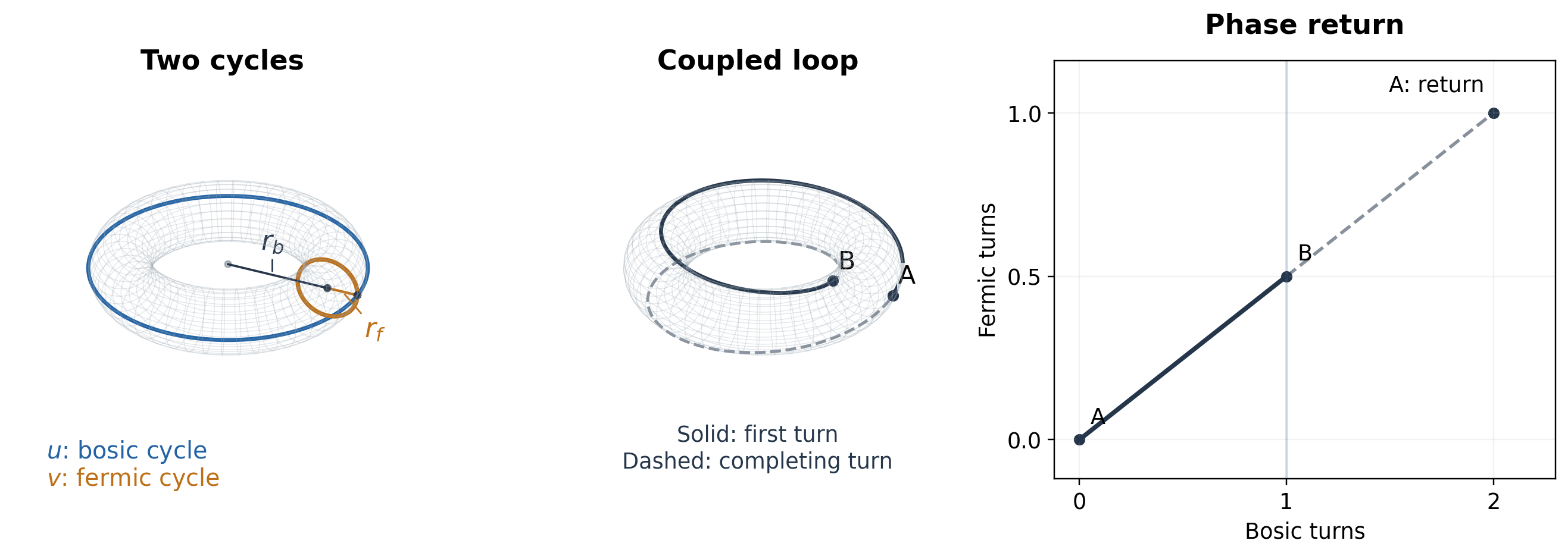
The surface path in Figure 6.1 couples the two advances. Follow it from A. After one major turn, the marker has reached the opposite minor phase, B: it has come around the central opening but has not returned around the tube. After a second major turn, it completes the minor turn as well. The pair of phases returns to A.
This is a selected two-to-one resonance. Resonance here means that the two advances remain locked in a ratio that permits a combined return. Other ratios give other paths. A rational ratio closes after suitable whole numbers of turns; an irrational ratio does not return exactly under steady two-phase motion. The torus accommodates all of these possibilities. A physical model must determine which of them can persist.
The two-to-one example is useful because the incomplete first return is easy to see. Returning both phase coordinates tells us where the marker is; describing its orientation requires further information. For now, the closed curve records a simpler fact—two periodic coordinates can complete a shared cycle even when they complete different numbers of turns.
The drawing also gives each cycle a size. Write \(r_b\) for the major display radius and \(r_f\) for the minor display radius. Changing either alters the shape we see. Connecting those sizes to momentum requires an additional physical rule; the phase labels alone do not supply one. We can already use the torus to follow recurrence before making that further identification.
6.3 Momentum and a Moving Clock
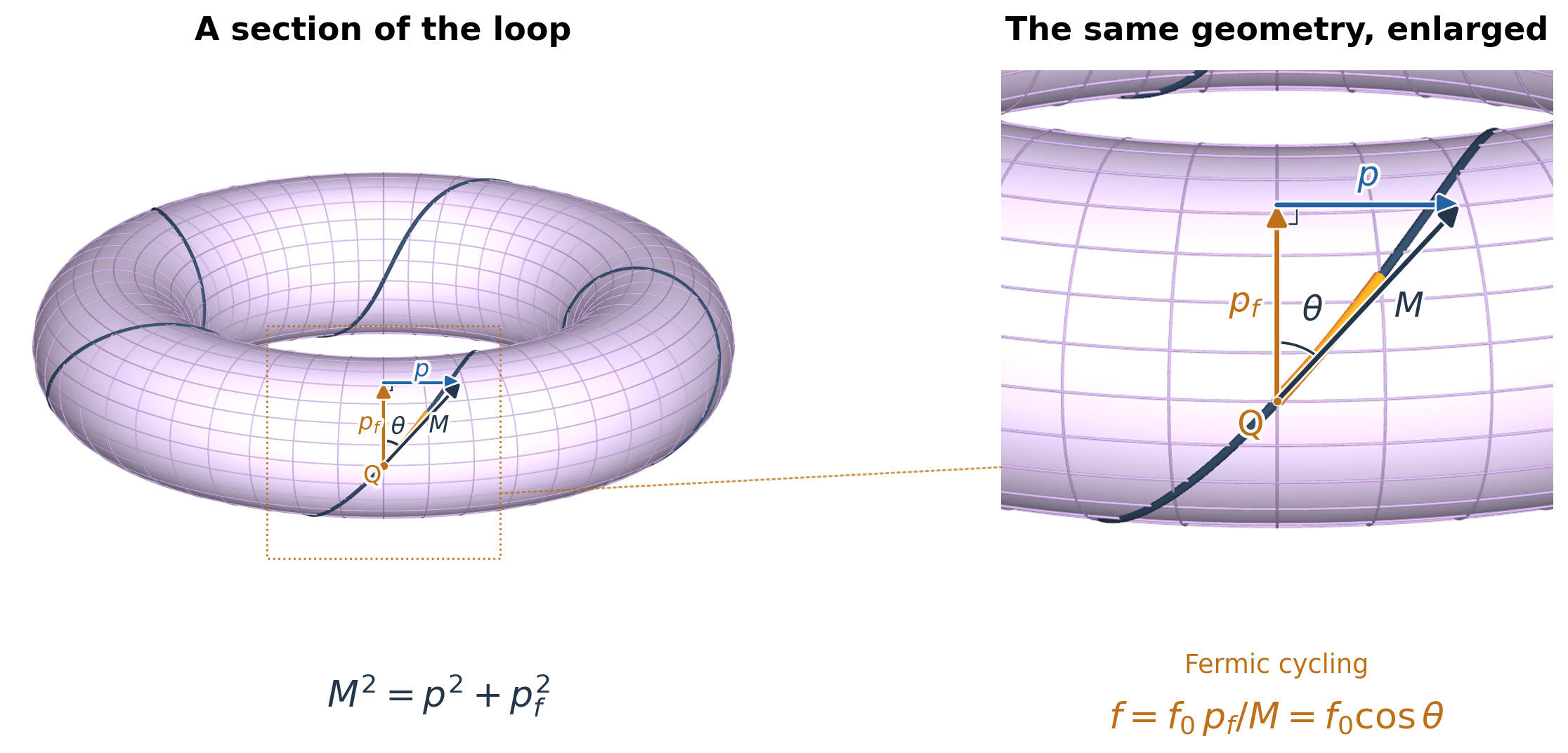
The two cycles organize the momentum of one carrier. Fermic momentum \(p_f\) supplies its stable internal scale, bosic momentum \(p\) its translational component, and core momentum \(M\) their combined magnitude. In the free inertial setting,
\[ M^2=p_f^2+p^2. \]
The triangle in Figure 6.2 makes this composition visible. At the front-centre point \(Q\), \(p_f\) and \(M\) share an origin, and the blue \(p\) arrow completes the triangle. Measure \(\theta\) from the fermic direction to \(M\): the fermic fraction is \(p_f/M=\cos\theta\), while the bosic fraction is \(p/M=\sin\theta\). The illustrated momentum ratio is chosen so that \(M\) follows the loop’s local tangent.
In the constant-speed manifold picture, propagation through the internal geometry maintains speed \(c\). The triangle resolves its direction into a fermic component \(c\cos\theta\) and a bosic component \(c\sin\theta\). Increasing bosic momentum at fixed \(p_f\) tilts the resultant away from the fermic direction. The underlying propagation speed stays fixed; its fermic component decreases.
A clock counts fermic cycles. Use reference time \(t\) in a chosen inertial frame. Let \(f_0\) be the carrier’s cycling frequency when at rest in that frame, and \(f\) its frequency when moving through it. Foundations gives the moving frequency as
\[ f=f_0\frac{p_f}{M}=f_0\cos\theta. \]
The moving carrier retains its fermic scale but completes fewer cycles during the same reference interval. At rest, \(p=0\), so \(M=p_f\), \(\theta=0\) and \(f=f_0\). As bosic momentum increases, \(M\) grows and the frequency falls. The changing angle pictures the slowing of a physical clock.
The same momentum balance governs translation. Choose an oriented direction \(\hat{k}\) in ordinary space. The signed component \(p_k=\vec p\cdot\hat{k}\) records the bosic momentum along it, and
\[ \dot x_k=c\frac{p_k}{M}. \]
The dot denotes change per unit reference time. Along the forward direction of motion, \(p_k=p\), so the translation speed is \(v=c\sin\theta\). The bosic fraction sets how quickly the carrier advances; the fermic fraction sets how quickly it cycles.
The moving clock records a time \(\tau\), calibrated so that each fermic cycle counts as \(1/f_0\). Counting the same cycles gives \(f\,dt=f_0\,d\tau\), hence
\[ d\tau=dt\,\frac{p_f}{M}. \]
Since \(v/c=p/M\), the momentum relation also gives \(p_f/M=\sqrt{1-v^2/c^2}=1/\gamma\), where \(\gamma\) is the Lorentz factor. This is the inertial time-dilation relation expressed through momentum and cycling.
The earlier two-to-one example showed when the two phases return together; the fermic frequency tells how quickly the clock cycles. To picture translation next, we follow the distance advanced during each bosic turn.
6.4 Translation and Pitch
Translation depends on the wave’s advance in the bosic direction and on how that advance is directed along the carrier’s motion. Write \(v_b\) for the wave velocity in the bosic direction. In the constant-speed manifold picture,
\[ v_b=c\sin\theta=c\frac{p}{M}. \]
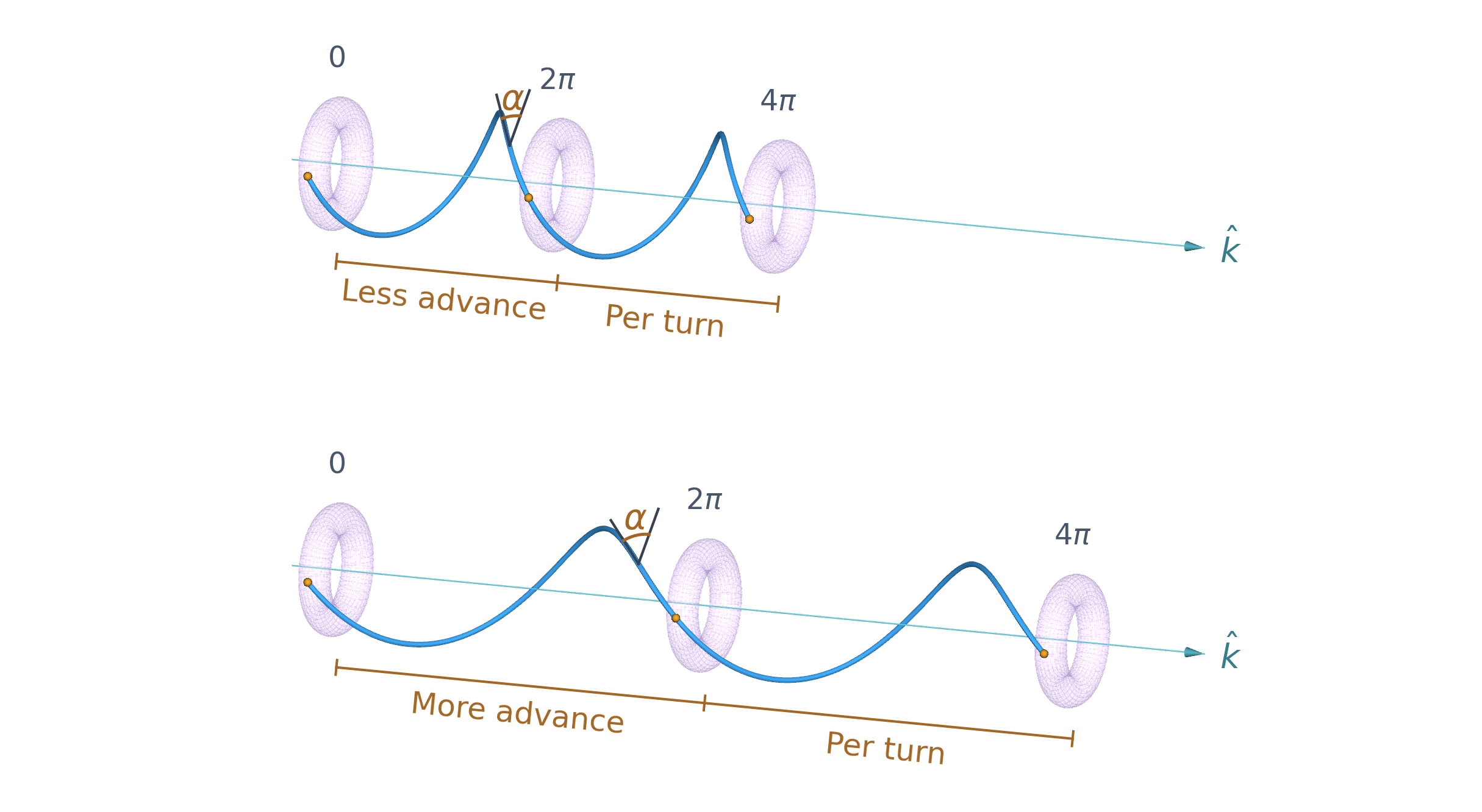
Keep the torus in view while the carrier translates. Place each turn of the bosic phase at the position the carrier has reached. Phase winds around the display axis while displacement advances along it, producing a helix. The torus’s symmetry axis is aligned with \(\hat{k}\), and its centre follows that straight axis. The helix records the bosic phase alone: its radius stays fixed rather than moving inward and outward with the fermic phase.
Define the pitch angle \(\alpha\) as the angle between the helix tangent and the circumferential direction in the plane perpendicular to \(\hat{k}\). The angle compares axial advance with advance around the bosic cycle. Use a calibrated helix picture in which those two distances share the same length scale. For steady motion along the forward branch,
\[ \dot x_k=v_b\tan\alpha. \]
Here \(v_b\) is the circumferential component, not the total speed along the drawn helix. A larger \(v_b\) gives faster translation at the same pitch angle; a larger \(\alpha\) gives faster translation at the same \(v_b\). The angles have different jobs: \(\theta\) resolves momentum into its fermic and bosic parts, while \(\alpha\) relates bosic advance to translation.
At \(\alpha=45^\circ\), axial and circumferential advances are equal. The translation law becomes
\[ \dot x_k=v_b=c\sin\theta=c\frac{p}{M}, \]
recovering the forward free-inertial relation. This \(45^\circ\) case belongs to the calibrated helix picture, rather than to an angle measured directly on the perspective drawing. For free inertial motion, \(v_b\) and \(\alpha\) must together satisfy the momentum law. Whether this equal-advance relation is fixed, or the bosic asymmetry can yield a smaller pitch angle in other circumstances, remains an open question.
Bosonic dilation changes the internal cycle’s extent and can also change its propagation and translation response. Cycle size alone therefore does not determine how quickly the carrier moves. The next section follows those changes together.
In the earlier two-turn example, the selected pair of phases returns after two bosic turns, but at a new position. Internal closure and return to the same place are different events. The distance advanced per turn is also distinct from a spatial wavelength, which compares equal wave phases at one instant. Identifying the two requires a relation between internal cycling and the spatial wave.
6.5 Two Ways to Dilate the Geometry
A cycle can grow in extent without changing how many times a pattern winds around it. Imagine spreading the same repeated pattern along a longer closed path. Each repetition then occupies more length. If the number of wave repetitions stays fixed and momentum scales inversely with their length, the corresponding momentum scale falls.
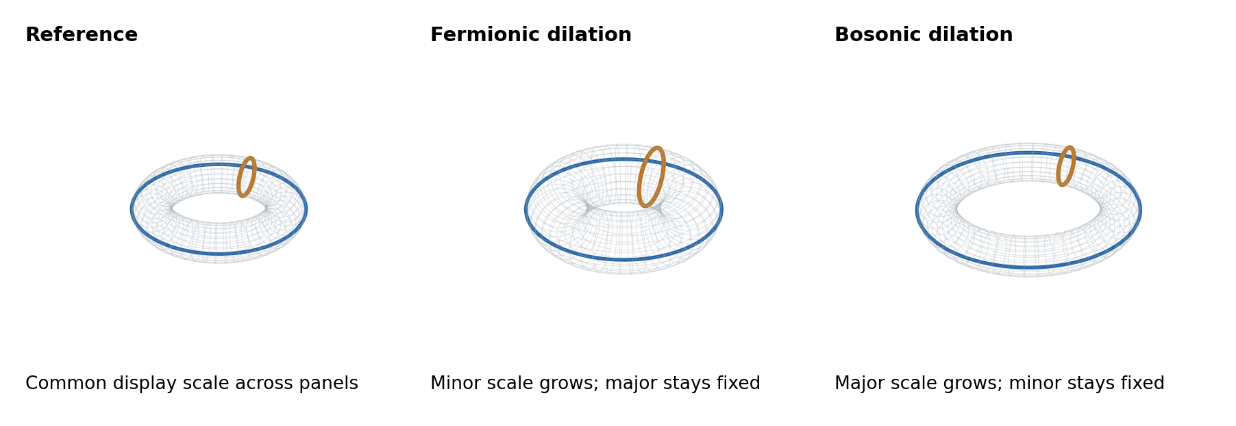
This supplies a useful conditional interpretation of the torus radii. Increasing the minor scale can depict a reduced fermic scale; increasing the major scale can depict a reduced bosic expression. The inverse-length rule is the extra assumption that connects the drawing to momentum. Without it, enlarging a torus is simply changing a picture.
6.5.1 Fermionic dilation and gravity
M1 interprets gravitational response through dilation of the internal fermionic geometry and the associated reduction of realized fermic momentum. The minor-cycle change in Figure 6.4 gives that interpretation a visible form. It must be read in the same comparison as the momentum change, rather than as a measured enlargement of a particle surface.
In the static, zero-shift comparison of the Gravity chapter, \(p_f\) denotes the particle’s fermic momentum in the free-space realization chosen as the reference. The temporal coefficient \(\phi^0{}_0\) of the deformation map expresses the gravitational change in that common reference:
\[ p_{f,r}=\phi^0{}_0p_f. \]
A value below one gives a smaller reference-expressed fermic scale. For the ideal clock held at rest in that chapter, the reference cycling rate falls by the same factor. The enlarged minor cycle is an illustration of the intended internal mechanism; the momentum and clock relations do not, by themselves, determine a unique physical radius.
A falling carrier must also obey its momentum budget. In the declared stationary free-fall comparison, its reference core \(M_r\) remains fixed while the reference-expressed fermic contribution falls and the bosic contribution grows. The torus’s internal change therefore belongs beside a changing translation history. It is not a loss of core momentum along that no-exchange trajectory. Stopping and settling the carrier is a separate interaction that transfers momentum to its surroundings.
6.5.2 Bosonic dilation and expansion
The Expansion chapter changes a different part of the organization. For a supplied homogeneous stage history, the factor \(\chi\) dresses the bosic contribution while the fermic scale remains fixed:
\[ M_\chi=\sqrt{p_f^2+\chi^2p^2}. \]
The conserved spatial momentum label is still \(p\); the bosic contribution to this generator is expressed as \(\chi p\). In the inverse-length picture, decreasing \(\chi\) corresponds to a longer bosonic cycle with the same number of repetitions. The major-radius change in Figure 6.4 illustrates that distinction: the bosonic geometry changes while the fermionic scale is held fixed.
Translation must follow the dressed generator as well. In the Expansion chapter’s true-frame coordinates, motion along the chosen direction obeys
\[ \dot x_k=\chi^2c\frac{p_k}{M_\chi}. \]
This is the coordinate translation rate; an observer using bound-frame rods expresses the motion in the corresponding local units. At the same conserved \(p\) and fermic scale \(p_f\), a smaller positive \(\chi\) gives a lower forward coordinate speed. The carrier advances less during an equal reference-time interval, even though the bosonic cycle is represented as larger.
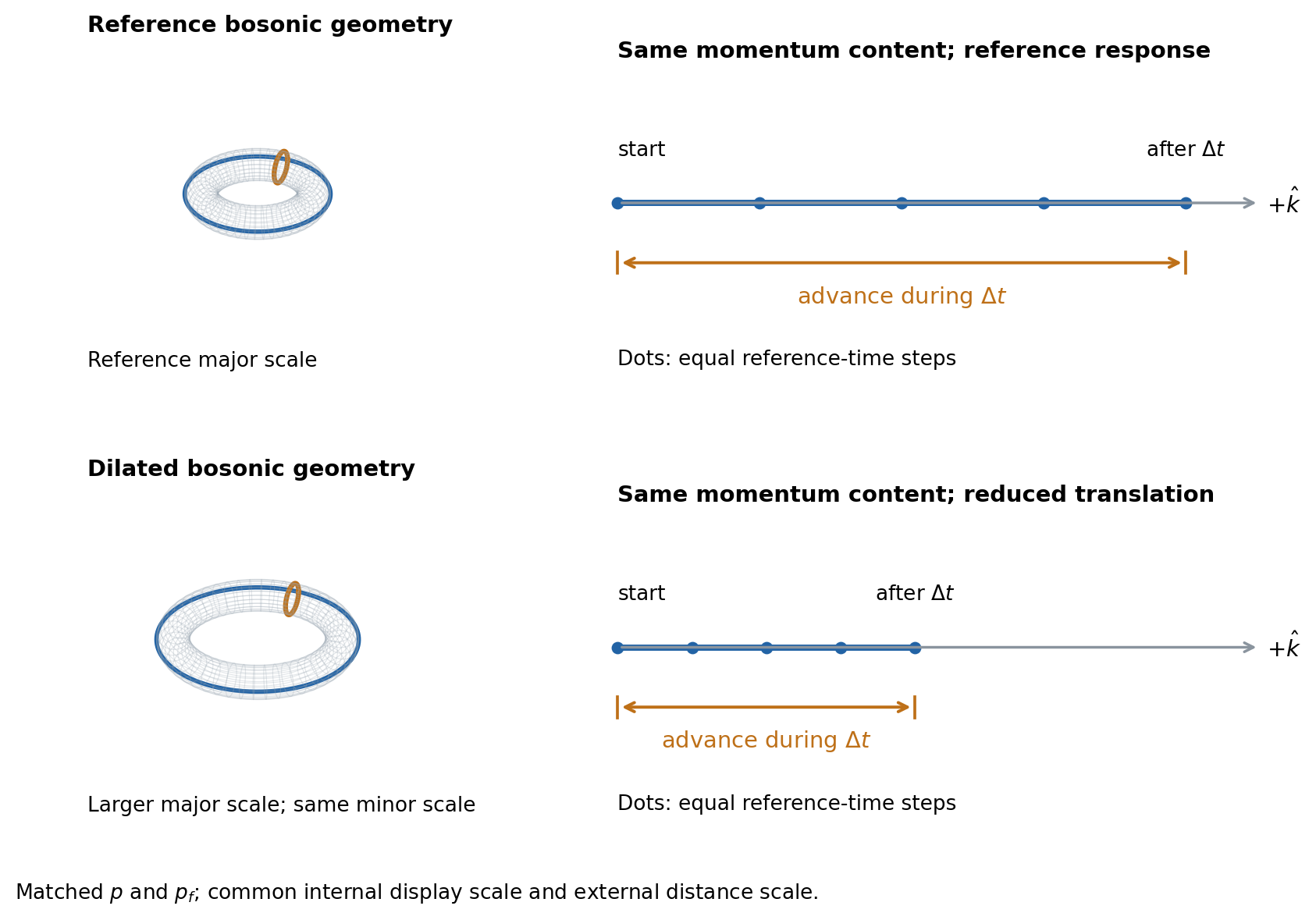
The two comparisons isolate different aspects of translation. Figure 6.3 follows a steady cycle and marks the advance per turn. Figure 6.5 changes the bosonic geometry while holding momentum content fixed, then compares advance per unit time. Assigning a helix to the second comparison would additionally require the bosic cycle’s period at each stage. Once that cadence is specified, the pitch follows from the same distance-per-cycle relation.
The two dilation pictures thus distinguish a gravitational change in the realized fermic scale from an expansion-driven change in the bosic contribution. Each changes a different part of the internal organization, with its effect governed by the corresponding momentum relations.
6.6 Resonant Loops and Waves
The closed path traced on the torus is a line. The surface provides a way to place its two phase coordinates, but the path itself can be followed without filling the surface. Seen this way, the resonance gives us a first string-like picture: a continuous loop winding through the two selected cycles.
There are two different changes we can now imagine. A marker can travel around the loop, recording progress through the resonant cycle. A pattern can also vary along the loop. To make the second idea visible, assign a scalar wave amplitude to each position and draw it as a colour. A crest is then a region of high amplitude, not a bulge in the torus surface.
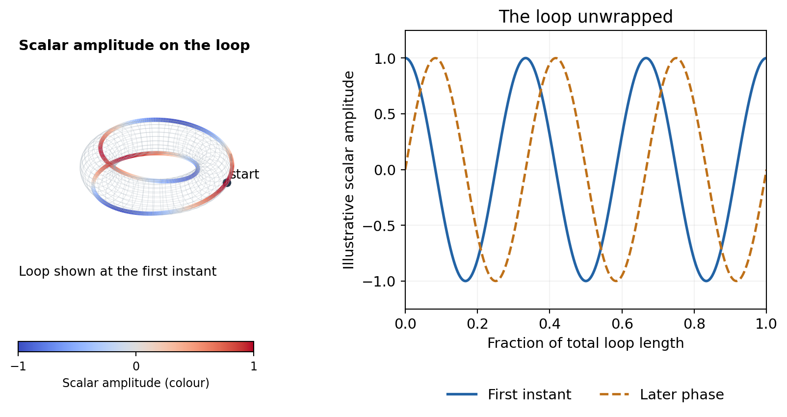
Because the loop closes, a continuous scalar pattern must agree where its end rejoins its beginning. In the simple periodic example of Figure 6.6, a whole number of wave repetitions fits around the loop. That number labels a mode. Stretching the loop while keeping the mode fixed increases the distance occupied by each repetition. This is the wave picture behind the inverse-length momentum interpretation used for dilation.
We can also make a mode visible through the shape itself. A deformation can vary around the major ring, making some tube sections broader and others narrower. It can also vary around the minor cycle, changing the shape of each section. The second variation makes the fermic amplitude visible across the tube rather than only around the ring. In the standing pattern below, both variations oscillate in place: the surface passes through its undeformed form, then the outward and inward displacements exchange.
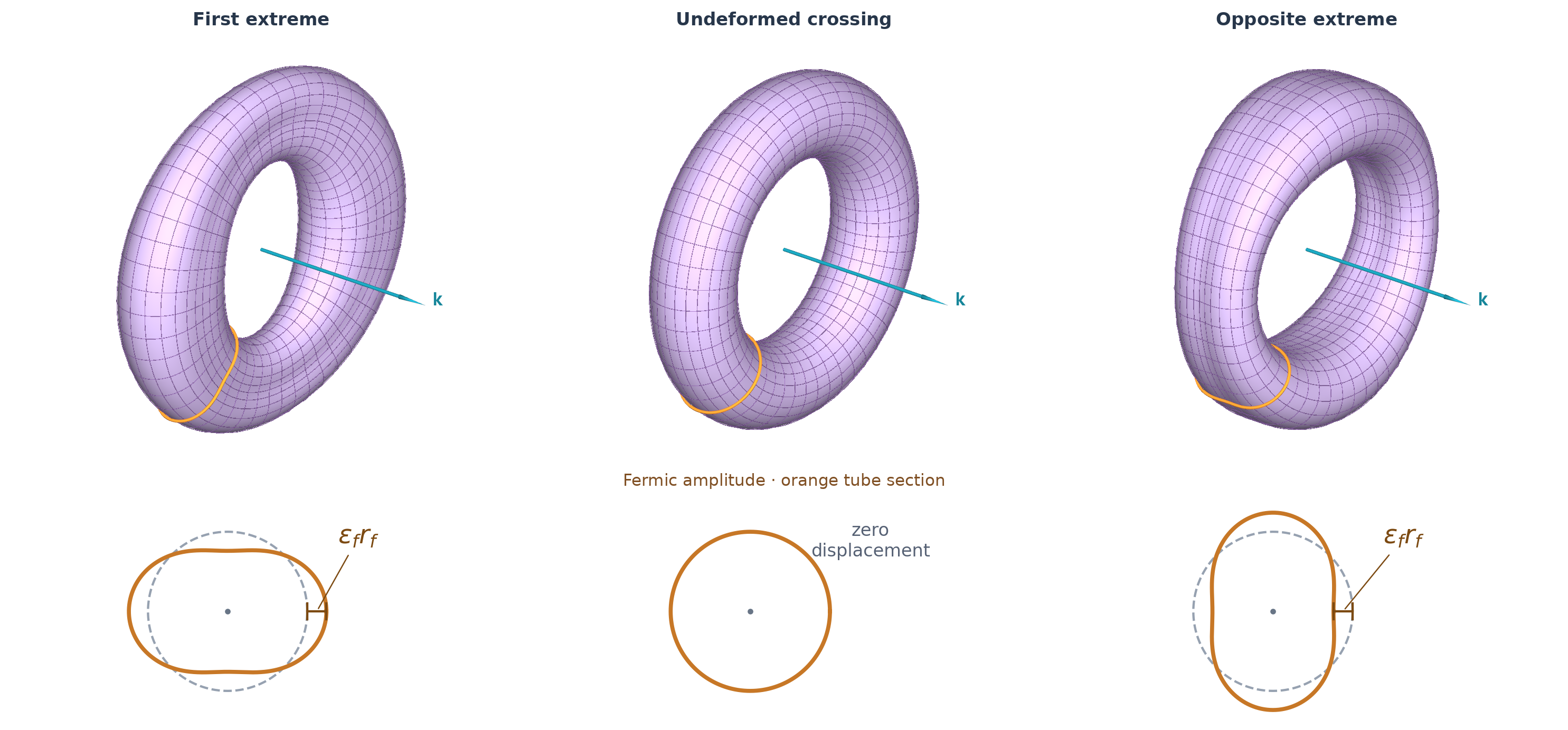
Unlike the colour pattern on the fixed loop, Figure 6.7 changes the geometry. Unlike the uniform dilation shown earlier, it makes one region larger while another becomes smaller. These are different questions about a cycle: how its overall scale changes, what pattern it carries, and whether that pattern deforms its shape.
A physical wave equation must determine which patterns propagate and which survive disturbances. More structured fields can also carry orientation information around the loop. Their return conditions need more than the single scalar amplitude used in these illustrations.
The same distinction matters for particle identity. A persistent particle would require an allowed internal organization that remains stable and has definite momentum and interaction properties. A winding number is a useful label for a pattern; it is not, on its own, an identification of that pattern with an electron or another species.
The loop prepares an equally useful question for string theory. Can an extended, phase-bearing object supply the dynamics that the torus picture leaves unspecified? To answer, we will have to compare what the object carries, what its allowed modes are and how it interacts. Calling the drawn loop a string is the beginning of that comparison, not its conclusion.
6.7 Beyond the First Picture
The torus has joined several relationships in one picture. Its two cycles keep the fermic and bosic momentum roles visible. Its resonant path shows internal return; the helix records translation during that return. Its two radii distinguish illustrative fermionic and bosonic dilation, and a pattern on the closed path gives waves somewhere to live.
Yet the same path can carry different wave patterns. Even a specified pattern can carry information the drawing has not shown: an orientation, a relative phase between components, or a rule for comparing it with another carrier. We can picture the first omission by attaching a small arrow to our moving marker. The marker may return to its starting point while the arrow has changed its orientation. Position on the torus no longer specifies the whole state.
Interactions make this additional information consequential. Two carriers can respond differently when their internal phases or orientations differ, even if their displayed radii and winding paths agree. A geometry capable of describing them must say how those states are compared across space and how their momentum changes through coupling. A bound rod or a material clock also requires such interactions; its behavior cannot be inferred by stretching a single torus drawing.
The next step keeps the two-cycle picture while adding the phase and orientation information needed to describe a fuller internal state. The Clifford torus provides a different geometric setting for two periodic coordinates, while Clifford algebra supplies the first-order representation of the momentum shell already encountered in quantum mechanics. Understanding their respective roles will let us ask how recurrence, orientation and translation can be described together—and what further dynamics makes that description a physical model.