4 Quantum Mechanics in Momentum Language
theoretical physics, foundations of physics, momentum conservation, canonical momentum, special relativity, stationary gravity, gravitoelectromagnetism, quantum mechanics, FLRW cosmology
4.1 Quantum momentum and interference
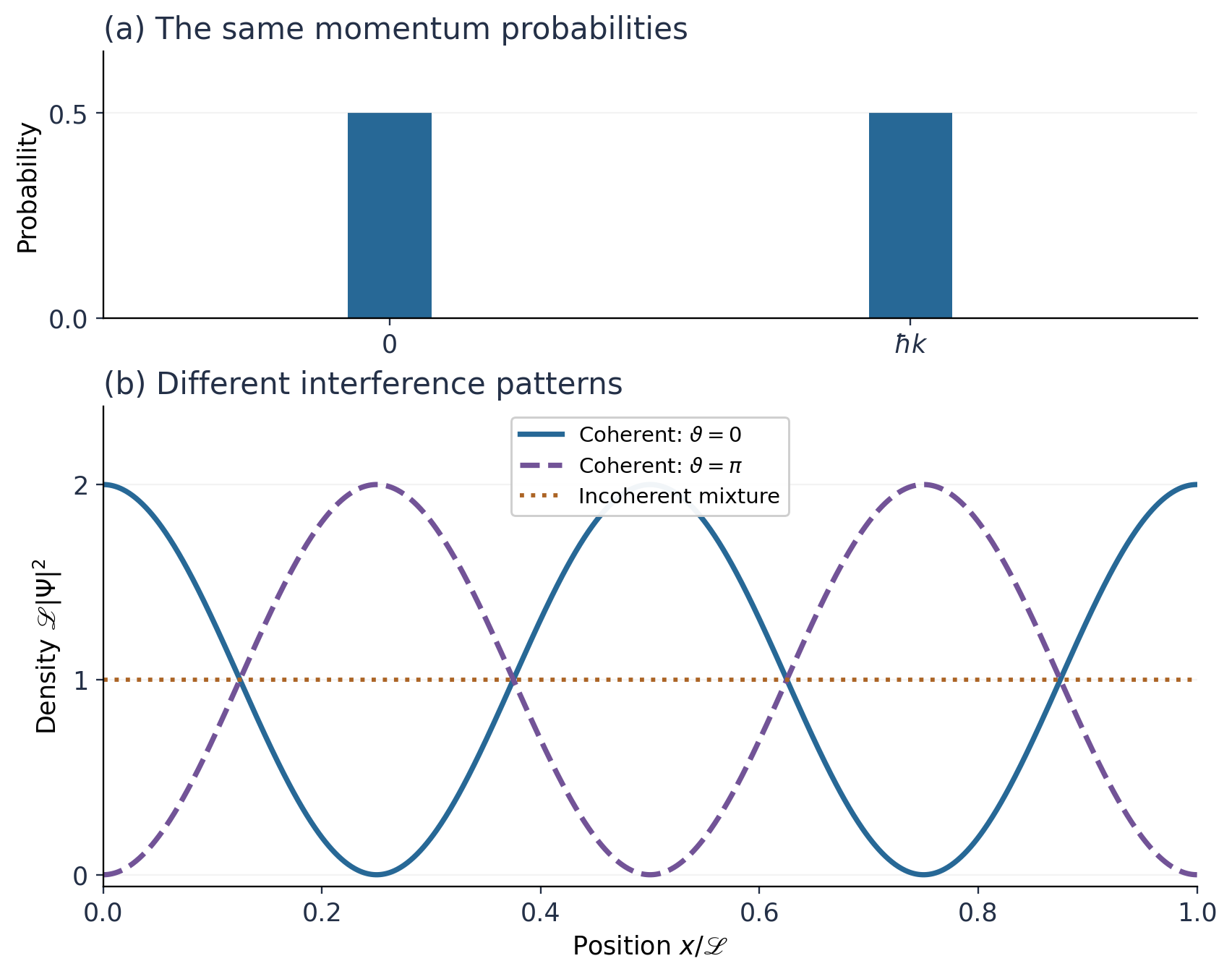
Two preparations can give the same momentum readings and still place their interference fringes in different positions. Take a coherent superposition of two momentum components. Changing their relative phase leaves the probability of either momentum unchanged, but moves the places where the amplitudes reinforce or cancel. A list of momentum probabilities therefore leaves out something physically observable.
The directional shell from Foundations and Gravity remains useful. It tells how a carrier’s common core and signed translation appear in opposed directions. Gravity then uses correlations between those components to distinguish, for example, transport along one axis from transport along another. Quantum mechanics adds a further requirement: a description must retain the phases that connect the momentum components of a state.
The object is now a phase-bearing state, \(\Psi\), rather than a trajectory with one definite momentum. Momentum operators act on its amplitudes, and an evolution generator advances their phases. M1 keeps the usual quantum state and probability rules while writing that generator in momentum units. The inherited shell supplies its free magnitude; a first-order spinor realization supplies a local wave equation.
Deformed space changes how that wave propagates and how its phase is compared. The same local and reference distinctions used for particles must therefore survive in the quantum equation. They also matter for a physical clock: a turning phase becomes a clock signal only when an observable internal process repeats.
The reverse gravitational question is just as important. A coherent state that responds to deformation must also enter a consistent account of the momentum that sources it. Its source can depend on interference, transport and internal stresses that no mean shell contains. The chapter develops the propagation and clock examples first, then uses them to make this reciprocal source problem precise.
4.2 Core Terms and Variables
The quantum state carries amplitudes and relative phases. Momentum operators act on that state; their possible readings and probabilities follow from the chosen measurement. The momentum shell keeps its earlier meaning, while the quantum description adds the information needed for interference.
4.2.1 State and evolution
| Symbol | Name and definition | Job |
|---|---|---|
| \(\Psi\) | Phase-bearing quantum state | Describes a coherent preparation, including its internal components. |
| \(\vartheta\) | Relative phase between two amplitudes | Controls how those amplitudes interfere. |
| \(\widehat A\) | An operator acting on the state | Represents a specified observable or generator; the hat distinguishes the operator from a scalar value. |
| \(\widehat M_t\) | Momentum-unit evolution generator: \((i\hbar/c)\partial_t\Psi=\widehat M_t\Psi\) in a fixed-norm representation | Generates phase change with respect to the selected time \(t\). |
Complex amplitudes, the Born probability rule and unitary evolution are the quantum premises used here. They are not consequences of the classical shell alone. The time coordinate is written \(x^0=ct\) when it is useful to give all four coordinates length units.
4.2.2 Free core and directional readings
| Symbol | Name and definition | Job |
|---|---|---|
| \(p_f\) | Fermic momentum of the declared free-space realization | Fixes the free massive shell; initially \(p_f>0\). |
| \(\widehat p_i=-i\hbar\partial_i\) | Signed spatial momentum operator in an inertial frame | Generates translations along axis \(i\). |
| \(\widehat M_+=\sqrt{p_f^2+\widehat{\mathbf p}^{\,2}}\) | Positive free core operator | Gives the positive magnitude associated with each free momentum component. |
| \(\widehat p^{i\sigma}=\widehat M_++\sigma\widehat p_i/2\) | Opposed directional reading operator, \(\sigma=\pm1\) | Combines common core and signed directional imbalance. |
| \(\beta,\alpha^i\) | Constant Hermitian spinor matrices | Supply the first-order realization developed in Section 4.4. |
Gravity’s slashed index \(\not i\) labels the six entries \((1+,1-,2+,2-,3+,3-)\). Its indexed \(L\) maps still convert between four- and six-component displays. The six reading labels describe momentum projections, not the number of components in \(\Psi\).
The subscript \(+\) on \(\widehat M_+\) marks a positive magnitude. The subscript \(t\) on \(\widehat M_t\) marks a generator’s time parameter. A first-order spinor generator has signed spectral branches; it agrees with the positive core on its free positive branch.
4.2.3 Gravity and comparison frames
| Symbol | Name and definition | Job |
|---|---|---|
| \(\phi^a{}_{\mu}\) | Gravity’s map: \(d\ell^a=\phi^a{}_{\mu}dx^\mu\) | Converts coordinate increments to local orthonormal components. |
| \(N=\phi^0{}_0\) | Temporal map coefficient in a Stage-adapted frame | Converts the normal local time increment to the selected coordinate normalization. |
| \(p_{{\mathrm{coord}},i}\), \(\widehat p_{{\mathrm{coord}},i}=-i\hbar\partial_i\) | Coordinate momentum and its derivative operator | Distinguishes a coordinate phase gradient from local momentum. |
| \(M\), \(p_{{\mathrm{local}},a}\) | Local core and local spatial momentum | Obey \(M^2=p_f^2+|\mathbf p_{\mathrm{local}}|^2\) for the free carrier. |
| \(M_r=NM\), \(p_{f,r}=Np_f\), \(\mathbf p_r=N\mathbf p_{\mathrm{local}}\) | Static, zero-shift reference-expressed momenta | Put the entire local shell into one common reference normalization. |
| \(M_t=-p_{{\mathrm{coord}},0}\) | Scalar chosen-time generator | Gives the future-branch phase rate; it equals \(M_r\) in the static zero-shift comparison. |
The symbol \(N\) abbreviates \(\phi^0{}_0\) in calculations. The coordinate label keeps the phase gradient distinct from local and reference-expressed momentum. Spatial variation also changes the volume used to normalize \(\Psi\). The construction in Section 4.5 introduces the corresponding representative \(\psi\) when that distinction becomes necessary.
4.3 Phase-bearing states and directional readings
Consider two momentum components in a periodic interval of length \(\mathscr L\). One has momentum zero; the other has momentum \(\hbar k\), where \(k\) is a nonzero allowed wave number. At one instant, a scalar Fourier representative with equal amplitudes is
\[ \Psi_\vartheta(x)=\frac{1+e^{i\vartheta}e^{ikx}}{\sqrt{2\mathscr L}}. \]
The relative phase is \(\vartheta\). A momentum measurement returns either value with probability one half, whatever \(\vartheta\) is. For the position measurement defined by this Fourier representation, however,
\[ |\Psi_\vartheta(x)|^2 =\frac{1+\cos(kx+\vartheta)}{\mathscr L}. \tag{4.1}\]
Changing the relative phase moves the interference fringes without changing either momentum weight. An incoherent preparation, which chooses one momentum or the other rather than superposing their amplitudes, has the same momentum weights but a uniform position distribution. Interference distinguishes the preparations.
4.3.1 Reading the inherited shell
For a free massive carrier in one inertial frame, each momentum component has the positive core \(M(\mathbf p)=\sqrt{p_f^2+|\mathbf p|^2}\). Acting on a superposition means applying this same rule to every momentum amplitude:
\[ \widehat M_+=\sqrt{p_f^2+\widehat{\mathbf p}^{\,2}},\qquad \widehat p^{i\sigma}=\widehat M_++\frac{\sigma}{2}\widehat p_i. \tag{4.2}\]
These are the quantum versions of the opposed readings already used in Gravity. Since \(M\geq|p_i|\), every reading is at least \(M/2\) and hence positive. The pair relations also survive as operator identities:
\[ \widehat p^{i+}+\widehat p^{i-}=2\widehat M_+,\qquad \widehat p^{i+}-\widehat p^{i-}=\widehat p_i. \]
All three pairs share the same core. The six entries are six projections of the same momentum organization, not six independently occupied states. Nor does their positivity make them probabilities: they have momentum units and are read through the state and its measurement rule.
In this free representation the reading operators are functions of the same commuting momenta. Consequently, even their complete joint probability distribution is unchanged when \(\vartheta\) changes in the two-component example. The directional display preserves the momentum information, but it does not restore the relative phase once that phase has been discarded.
4.3.2 Momentum spread and the shell of a mean
A superposition also requires care when taking averages. The shell holds for the operators,
\[ \widehat M_+^{\,2}-\widehat{\mathbf p}^{\,2}=p_f^2I, \]
so its expectation gives
\[ \langle\widehat M_+^{\,2}\rangle -\langle\widehat{\mathbf p}^{\,2}\rangle=p_f^2. \tag{4.3}\]
These are averages of squares, not squares of averages. To see the difference, take equal weights at opposite momenta \(\pm p_0\) along one axis. Both components have core \(M_0=\sqrt{p_f^2+p_0^2}\), while their mean signed momentum vanishes. Treating the mean list as a resting carrier would assign it the fermic scale \(M_0\) instead of \(p_f\). The missing information is the momentum spread: \(\langle p_x^2\rangle=p_0^2\).
The same example can be a coherent superposition or an incoherent mixture. Both share these momentum moments. Second moments repair the shell accounting, but they do not by themselves diagnose coherence.
A full directional representation can retain the phase by keeping correlations between different momentum arguments, together with the internal state components. Derivation 4.3A gives an invertible construction and the general covariance identity. In the main description, keeping \(\Psi\) makes the distinction immediate: momentum readings tell what values can be obtained; the coherent state also tells how their amplitudes interfere.
4.4 The core momentum operator
A momentum component must do more than satisfy the shell: it must also acquire the right phase as the state evolves. In the free positive-core description, the square-root operator supplies both jobs. A component with momentum \(\mathbf p\) has core \(M(\mathbf p)=\sqrt{p_f^2+|\mathbf p|^2}\) and evolves with the phase
\[ \Psi_{\mathbf p}(t)=e^{-icM(\mathbf p)t/\hbar}\Psi_{\mathbf p}(0). \]
Different momentum components generally turn through phase at different rates. Their relative phases then change, moving or reshaping the interference pattern. With the usual quantum phase calibration, the generator law is
\[ \boxed{\frac{i\hbar}{c}\partial_t\Psi=\widehat M_t\Psi.} \tag{4.4}\]
For free positive-core evolution, \(\widehat M_t=\widehat M_+\). A time-independent self-adjoint generator gives the unitary evolution \(\exp(-ic\widehat M_t t/\hbar)\), which preserves the state norm. The first derivative in time expresses phase evolution; it does not determine which spatial operator must generate it.
4.4.1 A local first-order realization
The square root is a legitimate operator. In momentum space it simply multiplies each amplitude by its core magnitude. In position space, however, it generally connects amplitudes at separated points rather than acting through a finite list of derivatives at one point. A local first-order equation requires a larger representation.
Dirac’s first-order construction (Dirac 1928), expressed in momentum units, keeps the fermic and directed bosic terms visible:
\[ \boxed{\widehat M_{t,\mathrm{flat}} =\beta p_f+\boldsymbol\alpha\cdot\widehat{\mathbf p}.} \tag{4.5}\]
Here \(\Psi\) is a four-component spinor, and the matrices \(\beta\) and \(\alpha^i\) act on its internal components. Their algebra is chosen so that squaring the generator recovers the shell:
\[ \beta^2=I,\qquad \{\beta,\alpha^i\}=0,\qquad \{\alpha^i,\alpha^j\}=2\delta^{ij}I. \]
The braces denote an anticommutator, \(\{A,B\}=AB+BA\). In the free case the spatial momentum operators commute, so
\[ \begin{aligned} \widehat M_{t,\mathrm{flat}}^{\,2} &=p_f^2I+p_f\{\beta,\alpha^i\}\widehat p_i +\tfrac12\{\alpha^i,\alpha^j\}\widehat p_i\widehat p_j\\ &=(p_f^2+\widehat{\mathbf p}^{\,2})I. \end{aligned} \tag{4.6}\]
The mixed fermic–bosic terms cancel. The remaining spatial terms combine into the squared momentum. This is the explanatory strength of the first-order form: a linear operator on amplitudes recovers the nonlinear scalar magnitude relation when squared.
The matrix choice is an explicit spinor realization of the shell. The six directional readings do not supply these spinor components or derive their statistics. They remain observables that can be expressed in either the four- or six-component momentum display.
4.4.2 Positive core and signed evolution
Squaring a number loses its sign. The same distinction matters here: at fixed momentum the first-order matrix has eigenvalues \(+M\) and \(-M\), while its magnitude is \(M\) on both branches. On the invariant free positive branch it agrees with \(\widehat M_+\). On the full spinor space it is a signed generator, not a positive core operator.
The enlarged representation makes the equation local. Restricting it to the positive branch requires a momentum-dependent projection, which is generally nonlocal in position space. These are two useful descriptions with different advantages: an explicitly positive free core, and a local first-order spinor equation.
A negative generator eigenvalue does not assign negative physical core to an antimatter particle. The opposite fermic-cycle orientation still carries positive core in M1; relating that orientation to particle and antiparticle field amplitudes requires the field description beyond this one-carrier construction.
Derivation 4.4A gives the spectral projections and the constrained six-component display. The free engine is now explicit: the state retains its amplitudes and relative phases, and a momentum-unit generator advances them while preserving the shell relation in its stated representation.
4.5 Quantum motion in deformed space
A wave packet crossing deformed space samples more than one local momentum comparison. Its phase accumulates against a chosen time standard, its spatial gradients are read through the map \(\phi\), and its spinor components must be compared between neighboring local frames. The simplest starting point is a static patch in which those conversions are constant.
4.5.1 One shell in local and reference descriptions
Take zero shift and an isotropic spatial map,
\[ \phi^0{}_0=N>0,\qquad \phi^a{}_i=b\delta^a{}_i,\qquad d\ell^0=Nc\,dt,\qquad d\ell^a=b\,dx^a. \]
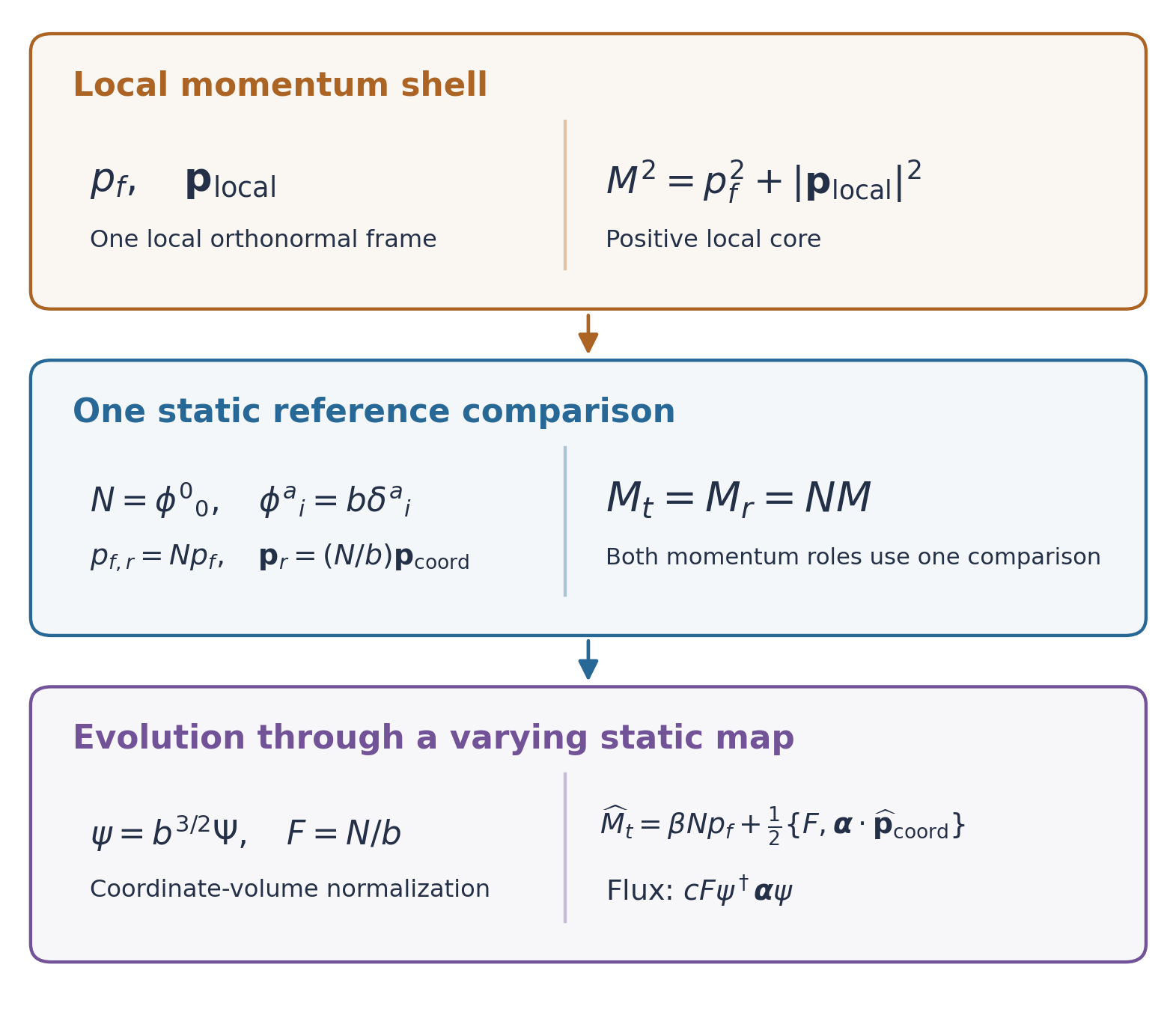
The scalar \(b>0\) gives the spatial conversion; it is distinct from Gravity’s indexed four/six maps \(L\). A coordinate phase gradient \(p_{{\mathrm{coord}},i}\) is read locally as \(p_{{\mathrm{local}},i}=p_{{\mathrm{coord}},i}/b\). The local core is therefore
\[ M=\sqrt{p_f^2+\frac{|\mathbf p_{\mathrm{coord}}|^2}{b^2}}. \]
The static reference expresses the whole shell with the common factor \(N\):
\[ p_{f,r}=Np_f,\qquad \mathbf p_r=\frac Nb\mathbf p_{\mathrm{coord}},\qquad M_r=NM=\sqrt{p_{f,r}^2+|\mathbf p_r|^2}. \tag{4.7}\]
A held particle has \(M_r=p_{f,r}\), just as in Gravity. During stationary free fall, \(M_r\) can remain constant while the local core \(M=M_r/N\) changes. The free local shell still contains \(p_f\); the reference shell contains \(Np_f\). Both describe the same carrier with different comparison standards.
In this constant patch the selected-time spinor generator is
\[ \widehat M_t=\beta Np_f+ \frac Nb\boldsymbol\alpha\cdot\widehat{\mathbf p_{\mathrm{coord}}}. \]
Its positive branch is \(NM=M_r\). Both terms have undergone the conversion required by the same clock and ruler comparison. Multiplying only the fermic term by \(N\) while leaving a local spatial derivative unchanged would mix those descriptions.
4.5.2 Spatial variation and probability flow
When \(N\) or \(b\) varies across the packet, a derivative also acts on the varying conversion factors. The shell magnitude alone no longer specifies the complete wave equation. We use a definite extension: the minimally coupled spinor equation, with neighboring spinors compared by the connection compatible with \(\phi\) and its metric. This supplies a prescribed-background quantum model; its microscopic M1 coupling remains to be derived.
Physical spatial volume is \(b^3d^3x\). Thus the norm of the original local spinor is \(\int b^3\Psi^\dagger\Psi\,d^3x\). It is convenient to absorb that volume factor into
\[ \psi=b^{3/2}\Psi,\qquad \int\psi^\dagger\psi\,d^3x=1. \]
The state has not changed; the representative now uses ordinary coordinate volume. In this representation the exact static isotropic generator is
\[ \boxed{ \widehat M_t=\beta Np_f+ \frac12\left\{\frac Nb, \boldsymbol\alpha\cdot\widehat{\mathbf p_{\mathrm{coord}}}\right\}. } \tag{4.8}\]
Writing \(F=N/b\) makes the derivative term transparent:
\[ \frac12\{F,\boldsymbol\alpha\cdot\widehat{\mathbf p_{\mathrm{coord}}}\} =F\boldsymbol\alpha\cdot\widehat{\mathbf p_{\mathrm{coord}}} -\frac{i\hbar}{2}\boldsymbol\alpha\cdot\nabla F. \]
The extra term records the variation of the conversion across the wave. It also makes the probability balance work. The equation for \(\psi\) gives
\[ \partial_t(\psi^\dagger\psi) +\nabla\cdot\left(cF\psi^\dagger\boldsymbol\alpha\psi\right)=0. \tag{4.9}\]
Probability leaving one region enters another. With appropriate decaying, periodic or reflecting boundary conditions, the total norm remains fixed. This current describes probability transport; it is not the gravitational momentum-source tensor.
4.5.3 Beyond the static isotropic patch
A general Stage-adapted map can also tilt the spatial frame relative to the coordinate time lines. Define its spatial part \(E^a{}_i=\phi^a{}_i\) and the shift \(w^i=(E^{-1})^i{}_a\phi^a{}_0\). Then
\[ d\ell^a=E^a{}_i(dx^i+w^ic\,dt),\qquad h_{ij}=\delta_{ab}E^a{}_iE^b{}_j. \]
The inverse spatial metric \(h^{ij}\) converts coordinate momentum into its local squared magnitude. For a future ray, the chosen-time generator becomes
\[ \boxed{M_t=N\sqrt{p_f^2+h^{ij}p_{{\mathrm{coord}},i}p_{{\mathrm{coord}},j}}-w^ip_{{\mathrm{coord}},i}.} \tag{4.10}\]
The shift contributes a drift relative to the coordinate grid. The full wave equation also carries the compatible spin transport. For example, in a rotating flat frame the coordinate generator contains both orbital and spin rotation; the shift alone supplies only the orbital part.
If the spatial volume changes with time, the representative \(\psi=(\det E)^{1/2}\Psi\) contributes a temporal derivative as well as spatial derivatives. These terms are fixed together by the same spinor equation. Derivation 4.5A constructs them and establishes probability-conserving evolution under its smooth-background and boundary assumptions. The local shell determines the leading momentum balance; the connection, ordering and volume measure determine how a coherent state travels through the varying geometry.
4.6 Phase and physical clocks
A moving wave packet accumulates phase while its peak travels through a spatial pattern. The phase change at a fixed position is therefore different from the phase change followed along the packet. Neither is automatically a clock reading: a clock must turn its internal evolution into an observable recurrence.
4.6.1 Following phase along a path
For a slowly varying packet write \(\Psi\simeq a e^{iS/\hbar}\), where \(S\) is the phase expressed in action units. Its spatial gradient gives the coordinate momentum, \(p_{{\mathrm{coord}},i}=\partial_iS\), and its time derivative gives \(\partial_tS=-cM_t\). This ray description applies when the amplitude and background vary slowly on the local wavelength scale, away from turning points and branch crossings.
Use the future generator from Equation 4.10. The packet velocity is \(\dot x^i=c\,\partial M_t/\partial p_{{\mathrm{coord}},i}\). Following the phase along that motion gives
\[ \begin{aligned} \frac{dS}{dt} &=\partial_tS+p_{{\mathrm{coord}},i}\dot x^i\\ &=-cM_t+p_{{\mathrm{coord}},i}\dot x^i\\ &=-\frac{cNp_f^2}{M}. \end{aligned} \tag{4.11}\]
The transport term subtracts the phase variation traversed by the packet. The shift cancels in the result. Along the same massive ray, \(d\tau/dt=Np_f/M\), so \(dS/dt=-cp_f\,d\tau/dt\).
In the static reference notation this becomes
\[ -\frac1\hbar\frac{dS}{dt} =\frac c\hbar\frac{p_{f,r}^{\,2}}{M_r}. \]
The magnitude agrees with Gravity’s ideal fermic-cycle rate. By contrast, the phase rate at a fixed coordinate is \(cM_t/\hbar\). For a null ray the leading phase is constant along the ray even though a detector at a fixed location can register an oscillating wave. Phase propagation and an internal fermic cycle are different physical comparisons.
4.6.2 A clock with an observable signal
A common phase multiplying an isolated state cancels from every expectation value. A clock signal instead needs a relative phase that changes a measured quantity. A two-state internal system supplies a simple example.
Call the two distinguishable configurations \(|L\rangle\) and \(|R\rangle\). Let their local momentum-unit generator be
\[ \widehat M_{\mathrm{int}}=M_0I+g\sigma_x,\qquad M_0>g>0, \]
where \(\sigma_x\) interchanges the configurations and \(g\) is the coherent coupling in momentum units. Its two stationary values are \(M_0\pm g\). Prepare the system in \(|L\rangle\) and hold it at rest in a zero-shift comparison, with \(N\) effectively uniform across its size. Assume that its internal dynamics couples to proper time without being altered by the support. Then
\[ \tau(t)=\int_0^tN(t')\,dt',\qquad |\Psi_{\mathrm{int}}(t)\rangle =e^{-icM_0\tau/\hbar} \left[ \cos\!\left(\frac{cg\tau}{\hbar}\right)|L\rangle -i\sin\!\left(\frac{cg\tau}{\hbar}\right)|R\rangle \right]. \]
The probability of finding the system in \(|R\rangle\) is
\[ \boxed{P_R(t)=\sin^2\!\left(\frac{cg\tau(t)}{\hbar}\right).} \tag{4.12}\]
The common \(M_0\) phase has disappeared. The gap \(2g\) produces the oscillation. Identically prepared trials measured after different waiting times reveal this signal without assuming that repeated measurements leave one running clock undisturbed.
At constant \(N\), the proper period is \(\pi\hbar/(cg)\) and the reference period is \(\pi\hbar/(cNg)\). A smaller \(N\) therefore gives a slower reference clock. The effect follows from the specified internal coupling, not from declaring every phase factor a clock.
4.6.3 What a common slowdown requires
One working clock does not establish that all material processes rescale together. A system can have several transition gaps, coherent couplings and relaxation rates. To behave as the same system running more slowly, all observable internal dynamics must share the time conversion.
Compare the baseline internal generator \(\widehat M_{{\mathrm{int}},0}\) with its reference-time counterpart \(\widehat M_{{\mathrm{int}},r}\). For a finite-dimensional closed sector with all states and observables accessible, every process shares one time rescaling exactly when
\[ \widehat M_{{\mathrm{int}},r} =\Lambda\widehat M_{{\mathrm{int}},0}+aI. \tag{4.13}\]
Here \(\Lambda\) is the common rate factor and \(aI\) changes only an unobservable common phase. Scaling one transition probability is weaker: it need not scale the coherent phase changes that drive other measurements. For an open system, relaxation and noise must be included in the comparison of the full dynamics.
Derivation 4.6A proves the criterion and separates the ray-phase identity from the internal-clock premise. The two-state example shows how a coherent quantum process can realize the gravitational clock comparison. Extending that result to material clocks requires their internal interactions and support conditions to produce the same rescaling.
4.7 Correspondence and controlled limits
The momentum-unit generator gives a common starting point for three familiar descriptions: relativistic spinor motion, a slow quantum envelope and an approximately classical trajectory. Each uses the same state dynamics at a different level of resolution. A matched barrier experiment then tests whether a gravitational comparison has changed the physical experiment or only its normalization.
4.7.1 Dirac dynamics in standard units
Multiplication by \(c\) converts the chosen-time generator into the conventional energy-unit Hamiltonian:
\[ \widehat H=c\widehat M_t. \]
For the flat first-order realization, using \(p_f=m_0c\) gives
\[ \widehat H =\beta m_0c^2+c\boldsymbol\alpha\cdot\widehat{\mathbf p}, \qquad i\hbar\partial_t\Psi=\widehat H\Psi. \]
This is the free Dirac equation in Hamiltonian form. The correspondence is exact: the amplitudes, phase evolution and measured probabilities are unchanged. Core momentum remains the primary quantity in the M1 description; energy units provide the familiar comparison.
4.7.2 The slow envelope
At low directed momentum, most of the free phase rate comes from the fermic scale. The positive magnitude expands as
\[ M=p_f+\frac{p^2}{2p_f}-\frac{p^4}{8p_f^3} +O\!\left(\frac{p^6}{p_f^5}\right). \]
The first term produces a rapid common rest phase. The slower change of the wave envelope is governed by the excess above it. In the standard Dirac block representation, write
\[ \Psi=e^{-icp_ft/\hbar}\binom{\varphi}{\xi}, \]
where \(\varphi\) and \(\xi\) are two-component amplitudes. The three Pauli matrices \(\boldsymbol\sigma\) act on these components. In the low-momentum positive branch, \(\xi\) is small. Its leading equation gives
\[ \xi\simeq\frac{\boldsymbol\sigma\cdot\widehat{\mathbf p}}{2p_f}\varphi. \]
Substituting into the equation for \(\varphi\) multiplies two first-order momentum operators. Since the free momentum derivatives commute, \((\boldsymbol\sigma\cdot\widehat{\mathbf p})^2=\widehat{\mathbf p}^{\,2}\), and
\[ \boxed{ \frac{i\hbar}{c}\partial_t\varphi =\frac{\widehat{\mathbf p}^{\,2}}{2p_f}\varphi. } \tag{4.14}\]
In energy units this is \(i\hbar\partial_t\varphi=-\hbar^2\nabla^2\varphi/(2m_0)\). The familiar second-order Schrödinger operator appears because the small spinor component has been eliminated, not because the underlying relativistic equation has changed its spatial order.
A weak, smooth static deformation adds the expected leading potential. Write \(N=\phi^0{}_0=1+\nu\) and take \(\nu\) and \(b-1\) to be of the same small order as \(p^2/p_f^2\), with spatial gradients controlled on the envelope scale. Removing the constant free rest phase then gives
\[ \frac{i\hbar}{c}\partial_t\varphi \simeq\left[p_f\nu+ \frac{\widehat{\mathbf p}_{\mathrm{coord}}^{\,2}}{2p_f}\right]\varphi. \]
For the Newtonian comparison, \(\Phi=c^2\nu\) turns the first term into \(m_0\Phi\) after multiplication by \(c\). Away from this weak, slowly varying regime, the ordered spinor equation must be used before reducing the envelope. In a constant isotropic patch, for example, the kinetic excess in reference units is \(N|\mathbf p_{\mathrm{coord}}|^2/(2p_fb^2)\): the same temporal conversion multiplies the whole local excess.
Derivation 4.7A supplies the elimination, gradient ordering and approximation conditions.
4.7.3 From waves to trajectories
The ray form used for the path-phase calculation also recovers particle motion. When \(\Psi\simeq a e^{iS/\hbar}\), derivatives acting on the rapidly varying phase dominate those acting on the amplitude. The spinor equation then requires
\[ g^{\mu\nu}\partial_\mu S\,\partial_\nu S=-p_f^2, \qquad g=\phi^{\mathsf T}\eta\phi. \tag{4.15}\]
Its future branch is the chosen-time generator already obtained from the momentum map. The rays follow
\[ \dot x^i=c\frac{\partial M_t}{\partial p_{{\mathrm{coord}},i}}, \qquad \dot p_{{\mathrm{coord}},i}=-c\frac{\partial M_t}{\partial x^i}. \]
Thus the same wave equation returns Gravity’s free-carrier trajectories. The compatible connection transports amplitude and spin at the next order. Near a turning point, where a propagating wave becomes an evanescent one, the simple ray approximation must give way to wave matching.
4.7.4 Matched gravitational barriers
Tunnelling is sensitive to small changes in the forbidden momentum because that momentum enters an exponential. It is therefore also sensitive to comparing different incident states or different apparatus standards by mistake.
Begin with a constant \(N\) and use proper distance \(\ell\) across a one-dimensional barrier. Let \(u(\ell)\) be its local additive momentum coefficient and \(C\) the stationary reference generator value. The local incident value is \(\epsilon=C/N\). Dividing the consistently converted stationary equation by \(N\) gives
\[ \left[-i\hbar\alpha^1\partial_\ell+\beta p_f+u(\ell)I\right]\psi =\epsilon\psi. \]
The temporal map coefficient has disappeared. Two experiments with the same local incident value, local barrier height, proper width, fermic scale and apparatus therefore have the same transmission. The incoming and outgoing probability fluxes must also be normalized in that same comparison. Derivation 4.7A checks the statement by exact spinor matching, without relying on a tunnelling exponent alone.
A spatially varying \(N\) is a different experiment. If the distant incident value \(C\) is held fixed, the local value \(C/N(\ell)\) changes along the barrier. In a forbidden interval the local decay momentum satisfies
\[ \kappa_{\mathrm{local}}^{\,2} =p_f^2-\left[\frac{C}{N(\ell)}-u(\ell)\right]^2. \]
Where the variation is slow enough for a semiclassical approximation, the amplitude contains
\[ \exp\!\left[-\frac1\hbar \int\kappa_{\mathrm{local}}\,d\ell\right]. \]
Nonuniform deformation can consequently change the transmitted fraction substantially. The appendix verifies such a change with the full wave equation and conserved flux. It is the gravitational sensitivity of the specified, consistently coupled spinor model, shared by its metric description. An additional quantum-gravitational effect would require an additional physical interaction, compared with the same preparation and apparatus—not a conversion applied to only one term of the shell.
4.8 Quantum sources and reciprocal gravity
A coherent carrier both responds to deformed space and contributes momentum to its source. The propagation equation describes the first direction. The second requires a local account of core, transport and stress that preserves the state’s interference and the momentum exchanged with other systems.
Gravity already supplied a simple reason to keep correlations. Equal counterstreams along \(x\) and equal counterstreams along \(y\) can have the same total core and zero net spatial momentum. Their six mean directional readings then agree, but their transport differs. Products of readings on each carrier retain that difference; products of the aggregate means lose it.
4.8.1 Correlate before averaging
For the free positive-core quantum description, the corresponding kinetic operator is
\[ \widehat j_{\mathrm{kin}}^{\not i\not j} =\widehat p^{\not i}\widehat M_+^{-1}\widehat p^{\not j}. \tag{4.16}\]
The inverse core weights the two directional readings on the same carrier. In an incoherent kinetic ensemble, summing these products with weights per physical volume returns Gravity’s source \(J^{\not i\not j}\). It is a momentum-weighted correlation, not an ordinary covariance.
The shell fixes its contraction before averaging:
\[ -\eta_{\not i\not j} \left\langle\widehat j_{\mathrm{kin}}^{\not i\not j}\right\rangle =p_f^2\left\langle\widehat M_+^{-1}\right\rangle. \tag{4.17}\]
The average inverse core appears here, rather than the inverse of the average core. Each momentum component brings its own weight. This is another place where replacing a distribution by a mean shell changes the source.
The reference conversion must preserve that weight too. For a static comparison at one common \(N=\phi^0{}_0\),
\[ \frac{p^{\not i}p^{\not j}}{M} =\frac{p_r^{\not i}p_r^{\not j}}{NM_r}. \]
The numerator contains two reference factors, while the core denominator contains one. The remaining factor of \(N\) restores the original local source. Conversion of physical volume is a separate step.
4.8.2 Interference enters the local source
The kinetic expression still leaves out a distinction exposed by the two-component state. Its momentum weights stay fixed when the relative phase changes, but its spatial interference pattern moves. A local coherent source can depend on the cross terms between those amplitudes as well as on their separate weights.
To calculate that source, the model must say how the coherent amplitudes couple to deformation. A specified matter action is one way to give propagation and source together: varying the matter state gives its equation of motion, while varying the deformation gives the momentum source. The action here is the mathematical rule for their joint dynamics. A free shell or a table of diagonal readings does not select that rule.
A scalar example makes the additional content concrete. Take a normalized free complex scalar state \(\Psi\) with positive-core evolution. To carry the inverse-core weighting into its quadratic source, form \(\zeta=\widehat M_+^{-1/2}\Psi\). This re-encodes the same state, retaining its relative phases. The minimally coupled quadratic scalar action specified in Derivation 4.8A acts on \(\zeta\).
Write this scalar model’s source as \(J_0^{\mu\nu}\). In its flat free realization, the local components are \(u=J_0^{00}\), \(j_i=J_0^{0i}\) and \(s_{ij}=J_0^{ij}\): common core density, core flux and momentum transport. They satisfy \(|\mathbf j|\leq u\), so the opposed densities are
\[ \boxed{d^{i\pm}=u\pm\frac12j_i\geq\frac u2\geq0.} \tag{4.18}\]
All pairs share the same local core. The scalar equation also gives their directional balance,
\[ \partial_0d^{i\pm} +\partial_j\left(j_j\pm\frac12s_{ji}\right)=0, \qquad x^0=ct. \]
For the normalized scalar state, with periodic or decaying boundaries, the integrated densities equal the expectation values of the free directional reading operators. Spatial phase is retained, and the transport terms carry changes between neighboring regions.
Those transport terms include gradients produced by interference. They can contain a negative transverse stress even while the common core and all opposed densities remain positive. A sum of nonnegative classical terms \(p_i^2/M\) cannot reproduce that stress. Thus a coherent source can satisfy positive directional balance without being a classical collection of independently moving carriers at every point.
4.8.3 Probability, total core and local source
The spinor model used for propagation has a different source. For its standard minimally coupled symmetric source, interference between two positive-branch modes can produce a negative local core-density patch. The probability density remains positive, and the spatially integrated core remains positive. Derivation 4.8A gives an explicit two-mode state exhibiting all three properties.
There is no contradiction between this example and the scalar construction. They use different matter models and different source expressions. Together they show why a positive probability, a positive total core and a positive local source are separate requirements. Writing the source in six components preserves its information; it cannot change a negative common-core value into six positive opposed densities.
Even a successful free scalar source is not uniquely fixed by its kinetic limit. Additional coherent gradient terms can leave the free diagonal readings and integrated totals unchanged while altering the local stress. Their physical selection must come from the interaction and the way its source is measured.
4.8.4 Complete reciprocal accounting
An interaction transfers momentum between participants and can entangle their internal states. The complete source must include that interaction and the systems that support or drive it. Counting only the responding carrier omits part of the exchange; counting the same interaction in both carriers’ cores counts it twice.
A finite two-carrier example in Derivation 4.8A demonstrates coherent entanglement with equal and opposite momentum transfer and positive conserved global directional charges. It is a constructive accounting example, not a derived local gravitational interaction. A native continuum description must supply the local source, its reciprocal response and the deformation dynamics within one common balance.
The quantity associated with internal recurrence also must not be mistaken for the entire gravitational source. Gravity’s source blocks give
\[ -\eta_{\not i\not j}J^{\not i\not j} =\mathcal M-\operatorname{tr}\mathcal C, \]
whereas the weak temporal deformation responds to \(\mathcal M+\operatorname{tr}\mathcal C\). A null kinetic carrier has zero fermic-recurrence contraction but a nonzero temporal source. Momentum does not need a fermic clock to gravitate.
A complete coherent interaction must determine both the response to deformation and its source, with material and Stage contributions included in the same directional balance.
4.9 A changing Stage and the one-particle boundary
A spatially uniform change of the Stage can alter phase evolution without changing a carrier’s spatial momentum label. Translation symmetry preserves that label. The changing Stage alters how the same directed content enters the generator.
The homogeneous case used by Expansion leaves the fermic scale fixed and supplies a positive bosic translation yield \(\chi(t)\). Its first-order generator is
\[ \boxed{\widehat M_\chi =\beta p_f+\chi(t)\boldsymbol\alpha\cdot\widehat{\mathbf p}.} \tag{4.19}\]
Here \(\mathbf p\) is the conserved spatial label used in Chapter 5. In the coordinate notation of Section 4.5 it is \(\mathbf p_{\mathrm{coord}}\). The same operator follows from the homogeneous map \(\phi^0{}_0=1\), \(\phi^a{}_i=\chi^{-1}\delta^a{}_i\), with zero shift and the volume-rescaled state. The connection and changing-volume terms combine as derived in Derivation 4.5A.
At fixed time, the positive branch magnitude is
\[ M_\chi=\sqrt{p_f^2+\chi^2p^2}. \]
For a narrow packet that follows this branch, its translation along axis \(k\) is
\[ \boxed{\dot x_k =c\frac{\partial M_\chi}{\partial p_k} =\chi^2c\,\frac{p_k}{M_\chi}.} \tag{4.20}\]
The two factors of \(\chi\) follow from differentiating the dressed squared momentum. The conserved label \(\mathbf p\) continues to represent the same spatial momentum content. Its local expression \(\mathbf p_{\mathrm{local}}=\chi\mathbf p\), phase rate and coordinate translation change with the Stage. The history \(\chi(t)\) is supplied here; deriving it requires the Stage’s dynamics and its complete source.
4.9.1 Following an instantaneous branch
A unitary equation preserves the full state norm, but a changing generator need not preserve its instantaneous positive branch. For a massive mode, changing \(\chi\) changes the relative weight of the fermic and bosic matrices. It therefore changes their eigenvectors as well as their eigenvalues.
If the change is slow compared with the separation of the spectral branches, and transitions remain small over the interval, a packet can approximately follow one branch. A rapid change can instead mix the instantaneous branches while conserving the full norm. Derivation 4.5A provides both a sudden-change example and the conditions for a controlled slow-history approximation. Particle creation cannot be inferred from this mixing alone; that interpretation requires a field state and a specified particle measurement.
4.9.2 Beyond a fixed carrier
A one-carrier state retains momentum and internal coherence within a fixed particle description. A field state can also contain coherence between different particle-number sectors, including the vacuum and a particle pair. That information is absent from a one-carrier density operator.
The distinction limits what can be inferred from positive one-carrier source examples. If a source operator were positive in every field state and had exactly zero vacuum expectation, it would annihilate the vacuum. It could then have no matrix element connecting the vacuum to a pair. A source with such pair coherence cannot satisfy all of those conditions at once. The vacuum source mean, its fluctuations and a detector’s response must therefore be distinguished rather than identified with one positive density.
Real unbound momentum can still source gravity without forming a stable particle. Waves and propagating spatial deformation already make that possibility part of the physical picture. A fluctuation variance, however, does not by itself establish additional positive mean core. A field description must determine the source and its measurement together.
For the supplied homogeneous history, the packet law above gives a concrete next step. Chapter 5 follows massive and lightlike propagation and compares emitted patterns with material standards at a later epoch. A quantum law for the Stage and a complete field-source theory remain separate tasks.
4.10 What the quantum chapter establishes
A coherent momentum state carries more than a list of possible readings. Its amplitudes and relative phases determine interference, while its momentum operators preserve the directional shell and its second-moment balance. The six-component display makes common core and opposed imbalance visible without replacing the state that connects them.
Core momentum also organizes quantum evolution. The positive free magnitude and the local first-order spinor generator give complementary representations, with agreement on the free positive branch. Consistent conversion through \(\phi\) extends the specified spinor model to deformed space, including the derivative ordering, spin transport and volume factors needed for probability conservation. Its slow envelope and rays recover the corresponding Schrödinger and gravitational particle limits; matched barriers distinguish physical spatial variation from a change of normalization.
A coherent internal process can turn that evolution into a clock signal. Its observable recurrence depends on relative phase and a specified internal coupling. A reciprocal gravitational description asks more: the same interaction must determine the response and the complete coherent source. The scalar and spinor examples make that requirement sharper, but do not yet select the microscopic M1 interaction or a quantum law for the Stage.
The next chapter takes the homogeneous Stage history as supplied. It asks how conserved spatial momentum translates and how signals are compared when the bosic yield changes. The quantum generator now provides the link from that changing yield to phase and motion.